ICS 311 #5A: Probabilistic Analysis

Review Material

• ICS 141 (Counting)
• ICS 141 (Discrete Probabilities)
• CLRS Appendix C-1 through C-3.

Outline

1. Probabilistic Analysis
2. Indicator Random Variables
3. Expected Number of Inversions

Readings and Screencasts

• CLRS Sections 5.1-5.3
• Screencasts 5A, 5B (also in Laulima)

Probabilistic Analysis

Instead of limiting analysis to best case or worst case, we can analyze all cases based on a distribution of the probability of each case and compute the expected runtime based on this distribution.

For example, it is easy to show that given uniformly distributed random input it takes n/2 comparisons on average to find an item in a linked list of n items. This is an example of randomized analysis of the search algorithm in a linked list.

Hiring Problem and Cost

To illustrate probabilistic analysis, consider the following problem. Suppose you are using an employment agency to hire an office assistant.

• The agency sends you one candidate per day: interview and decide.
• Cost to interview is c_i per candidate (fee to agency).
• Cost to hire is c_h per candidate (includes firing prior assistant and fee to agency).
• c_h > c_i
• You always hire the best candidate seen so far.

  Hire-Assistant(n)
  1  best = 0                // fictional least qualified candidate
  2  for i = 1 to n
  3    interview candidate i // paying cost  ci
  4    if candidate i is better than candidate best
  5      best = i
  6      hire candidate i    // paying cost ch

What is the cost of this strategy?

• If we interview n candidates and hire m of them, cost is O(c_in + c_hm)
• We interview all n and c_i is small, so we focus on c_hm.
• c_hm varies with each run and depends on interview order
• This is a common paradigm: finding the maximum or minimum in a sequence by examining each element, and changing the winner m times.

Best Case

If each candidate is worse than all who came before, we hire one candidate:
    O(c_in + c_h) = O(c_in)

Worst Case

If each candidate is better than all who came before, we hire all n (m = n):
    O(c_in + c_hn) = O(c_hn) since c_h > c_i
But this is pessimistic. What happens in the average case?

Probabilistic Analysis

• We must know or make assumptions about the distribution of inputs.
• The expected cost is over this distribution.
• The analysis will give us average case running time.

We don't have this information for the Hiring Problem, but suppose we could assume that candidates come in random order. Then the analysis can be done by counting permutations:

• Each ordering of candidates (relative to some reference ordering such as a ranking of the candidates) is equally likely to be any of the n! permutations of the candidates.
• In how many do we hire once? twice? three times? ... n−1 times? n times?
• It depends on how many permutations have zero, one two ... n−2 or n−1 candidates that come before a better candidate.
• This is complicated!
• Instead, we can do this analysis with indicator variables (next section)

Randomized Algorithms

We might not know the distribution of inputs or be able to model it.

Instead we randomize within the algorithm to impose a distribution on the inputs.

An algorithm is randomized if its behavior is determined in parts by values provided by a random number generator.

This requires a change in the hiring problem scenario:

• The employment agency sends us a list of n candidates in advance and lets us choose the interview order.
• We choose to interview them in random order.

Thus we take control of the question of whether the input is randomly ordered: we enforce random order, so the average case becomes the expected value.

Probabilistic Analysis with Indicator Random Variables

Here we introduce technique for computing the expected value of a random variable, even when there is dependence between variables. Two informal definitions will get us started:

A random variable (e.g., X) is a variable that takes on any of a range of values according to a probability distribution.

The expected value of a random variable (e.g., E[X]) is the average value we would observe if we sampled the random variable repeatedly.

Indicator Random Variables

Given sample space S and event A in S, define the indicator random variable

We will see that indicator random variables simplify analysis by letting us work with the probability of the values of a random variable separately.

Lemma 1

For an event A, let X_A = I{A}. Then the expected value E[X_A] = Pr{A} (the probability of event A).

Proof: Let ¬A be the complement of A. Then

E[X_A] = E[I{A}]   (by definition)
    = 1*Pr{A} + 0*Pr{¬A}   (definition of expected value)
    = Pr{A}.

Simple Example

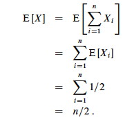
What is the expected number of heads when flipping a fair coin once?

• Sample space S is {H, T}
• Pr{H} = Pr{T} = 1/2
• Define indicator random variable X_H= I{H}, which counts the number of heads in one flip.
• Since Pr{H} = 1/2, Lemma 1 says that E[X_H] = 1/2.

Less Simple Example

What is the expected number of heads when we flip a fair coin n times?

Let X be a random variable for the number of heads in n flips.

We could compute E[X] = ∑_i=0,ni Pr{X=i} -- that is, compute and add the probability of there being 0 heads total, 1 head total, 2 heads total ... n heads total, as is done in C.37 in the appendix and in the screencast lecture 5A -- but it's messy!

Instead use indicator random variables to count something we do know the probability for: the probability of getting heads when flipping the coin once:

• For i = 1, 2, ... n define X_i = I{the ith flip results in event H}.
• Then X = ∑_i=1,nX_i.   (That is, count the flips individually and add them up.)
• Lemma 1 says that E[X_i] = Pr{H} = 1/2 for i = 1, 2, ... n.
• Expected number of heads is E[X] = E[∑_i=1,nX_i]
• Problem: We don't have ∑_i=1,nX_i; we only have E[X₁], E[X₂], ... E[X_n].
• Solution: Linearity of expectation (appendix C): expectation of sum equals sum of expectations. Therefore:
  

The key idea: if it's hard to count one way, use indicator random variables to count an easier way!

Hiring Problem Revisited

Assume that the candidates arrive in random order.

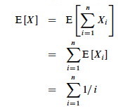
Let X be the random variable for the number of times we hire a new office assistant.

Define indicator random variables X₁, X₂, ... X_n where X_i = I{candidate i is hired}.

We will rely on these properties:

• X = X₁ + X₂ + ... + X_n   (The total number of hires is the sum of whether we did each individual hire (1) or not (0).)
• Lemma 1 implies that E[X_i] = Pr{candidate i is hired}.

We need to compute Pr{candidate i is hired}:

• Candidate i is hired iff candidate i is better than candidates 1, 2, ..., i−1
• Assumption of random order of arrival means any of the first i candidates are equally likely to be the best one so far.
• Thus, Pr{candidate i is the best so far} = 1/i.
  (Intuitively, as you add more candidates each candidate is less and less likely to be better than all the ones prior.)

By Lemma 1, E[X_i] = 1/i, a fact that lets us compute E[X]:

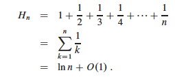
The sum is a harmonic series. From formula A7 in appendix A, the n^th harmonic number is:

Thus, the expected hiring cost is O(c_h ln n), much better than worst case O(c_hn)! (ln is the natural log. Formula 3.15 of the text can be used to show that ln n = O(lg n.)

We will see this kind of analysis repeatedly. Its strengths are that it lets us count in ways for which we have probabilities (compare to derivation of equation C.37 in the textbook), and that it works even when there are dependencies between variables.

Expected Number of Inversions

Here is another example of probabilistic analysis. This is Exercise 5.2-5 page 122, for which there is a publicly posted solution. This example shows the great utility of random variables.

Let A[1.. n] be an array of n distinct numbers. If i < j and A[i] > A[j], then the pair (i, j) is called an inversion of A (they are "out of order" with respect to each other). Suppose that the elements of A form a uniform random permutation of ⟨1, 2, ... n⟩.

We want to find the expected number of inversions. This has obvious applications to analysis of sorting algorithms, as it is a measure of how much a sequence is "out of order". In fact, each iteration of the while loop in insertion sort corresponds to the elimination of one inversion (see the posted solution to problem 2-4c).

If we had to count in terms of whole permutations, figuring out how many permutations had 0 inversions, how many had 1, ... etc. (sound familiar? :), that would be a real pain, as there are n! permutations of n items. Can indicator random variables save us this pain by letting us count something easier?

We will count the number of inversions directly, without worrying about what permutations they occur in:

Let X_ij, i < j, be an indicator random variable for the event where A[i] > A[j] (they are inverted).

More precisely, define: X_ij= I{A[i] > A[j]} for 1 ≤ i < j ≤ n.

Pr{X_ij = 1} = 1/2 because given two distinct random numbers the probability that the first is bigger than the second is 1/2. (We don't care where they are in a permutation; just that we can easily identify the probabililty that they are out of order. Brilliant in its simplicity!)

By Lemma 1, E[X_ij] = 1/2, and now we are ready to count.

Let X be the random variable denoting the total number of inverted pairs in the array. X is the sum of all X_ij that meet the constraint 1 ≤ i < j ≤ n:

We want the expected number of inverted pairs, so take the expectation of both sides:

Using linearity of expectation, we can simplify this far:
$$ \begin{align} E[X] &= E\left[\sum_{i=1}^{n-1} \sum_{j=i+1}^n X_{ij}\right] \\ &= \sum_{i=1}^{n-1} \sum_{j=i+1}^n E\left[X_{ij}\right] \\ &= \sum_{i=1}^{n-1} \sum_{j=i+1}^n \frac{1}{2} \\ &= \frac{1}{2} \sum_{i=1}^{n-1}\sum_{j=i+1}^n 1 \\ &= \frac{1}{2} \sum_{i=1}^{n-1} (n-i) \\ &= \frac{1}{2} \left(\sum_{i=1}^{n-1} n - \sum_{i=1}^{n-1}i\right) \\ &= \frac{1}{2} \left(n(n-1) - \frac{n(n-1)}{2}\right) \\ &= \frac{n(n-1)}{4} \end{align} $$

Therefore the expected number of inverted pairs is n(n − 1)/4, or O(n²).

Applications