
So far we have seen the following sorting algorithms: InsertionSort, MergeSort and HeapSort. We start these Lecture notes with another sorting algorithm: Quicksort. Quicksort, like Mergesort, takes a divide and conquer approach, but on a different basis.
If we have done two comparisons among three keys and find that x < p and p < y, do we ever need to compare x to y? Where do the three belong relative to each other in the sorted array?
Quicksort uses this idea to partition the set of keys to be sorted into those less than the pivot p and those greater than the pivot. (It can be generalized to allow keys equal to the pivot.) It then recurses on the two partitions.

Compare this to Mergesort.
Quicksort performs well in practice, and is one of the most widely used sorts today.
To sort any subarray A[p .. r], p < r:
An array is sorted with a call to QUICKSORT(A, 1, A.length):

The work is done in the PARTITION procedure. A[r] will be the pivot. (Note that the end element of the array is taken as the pivot. Given random data, the choice of the position of the pivot is arbitrary; working with an end element simplifies the code):

PARTITION maintains four regions.

Three of these are described by the following loop invariants, and the fourth (A[j .. r-1]) consists of elements that not yet been examined:
Loop Invariant:
- All entries in A[p .. i] are ≤ pivot.
- All entries in A[i+1 .. j-1] are > pivot.
- A[r] = pivot.
It is worth taking some time to trace through and explain each step of this example of the PARTITION procedure, paying particular attention to the movement of the dark lines representing partition boundaries.

Continuing ...

Here is the Hungarian Dance version of quicksort, in case that helps to make sense of it!
Here use the loop invariant to show correctness:
The formal analysis will be done on a randomized version of Quicksort (see below). This informal analysis helps to motivate that randomization.
First, PARTITION is Θ(n): We can easily see that its only component that grows with n is the for loop that iterates proportional to the number of elements in the subarray).
The runtime depends on the partitioning of the subarrays:
The worst case occurs when the subarrays are completely unbalanced, i.e., there are 0 elements in one subarray and n-1 elements in the other subarray (the single pivot is not processed in recursive calls). This gives a familiar recurrence (compare to that for insertion sort):

One example of data that leads to this behavior is when the data is already sorted: the pivot is always the maximum element, so we get partitions of size n−1 and 0 each time. Thus, quicksort is O(n2) on sorted data. Insertion sort actually does better on a sorted array! (O(n))
The best case occurs when the subarrays are completely balanced (the pivot is the median value): subarrays have about n/2 elements. The reucurrence is also familiar (compare to that for merge sort):

It turns out that expected behavior is closer to the best case than the worst case. Two examples suggest why expected case won't be that bad.
Suppose each call splits the data into 1/10 and 9/10. This is highly unbalanced: won't it result in horrible performance?

We have log10n full levels and log10/9n levels that are nonempty.
As long as it's constant, the base of the log does not affect asymptotic results. Any split of constant proportionality will yield a recursion tree of depth Θ(lg n). In particular (using ≈ to indicate truncation of low order digits),
log10/9n = (log2n) / (log210/9) by formula 3.15
≈ (log2n) / 0.152
= 1/0.152 (log2n)
≈ 6.5788 (log2n)
= Θ(lg n), where c = 6.5788.
So the recurrence and its solution is:

A general lesson that might be taken from this: sometimes, even very unbalanced divide and conquer can be useful.
With random data there will usually be a mix of good and bad splits throughout the recursion tree.
A mixture of worst case and best case splits is asymptotically the same as best case:

Both these trees have the same two leaves. The extra level on the left hand side only increases the height by a factor of 2, and this constant disappears in the Θ analysis.
Both result in O(n lg n), though with a larger constant for the left.
Instead of limiting analysis to best case or worst case, we can analyze all cases based on a distribution of the probability of each case and compute the expected runtime based on this distribution.
We implicitly used probabilistic analysis when we said that given random input it takes n/2 comparisons on average to find an item in a linked list of n items.
To illustrate probabilistic analysis, consider the following problem. Suppose you are using an employment agency to hire an office assistant.
  Hire-Assistant(n)
  1  best = 0                // fictional least qualified candidate
  2  for i = 1 to n
  3    interview candidate i // paying cost  ci
  4    if candidate i is better than candidate best
  5      best = i
  6      hire candidate i    // paying cost ch
What is the cost of this strategy?
If each candidate is worse than all who came before, we hire one candidate:
O(cin + ch) = O(cin)
If each candidate is better than all who came before, we hire all n (m =
n):
O(cin + chn) = O(chn) since
ch > ci
But this is pessimistic. What happens in the average case?
We don't have this information for the Hiring Problem, but suppose we could assume that candidates come in random order. Then the analysis can be done by counting permutations:
We might not know the distribution of inputs or be able to model it.
Instead we randomize within the algorithm to impose a distribution on the inputs.
An algorithm is randomized if its behavior is determined in parts by values provided by a random number generator.
This requires a change in the hiring problem scenario:
Thus we take control of the question of whether the input is randomly ordered: we enforce random order, so the average case becomes the expected value.
Here we introduce technique for computing the expected value of a random variable, even when there is dependence between variables. Two informal definitions will get us started:
A random variable (e.g., X) is a variable that takes on any of a range of values according to a probability distribution.
The expected value of a random variable (e.g., E[X]) is the average value we would observe if we sampled the random variable repeatedly.
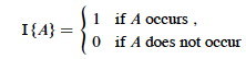
Given sample space S and event A in S, define the indicator random variable
We will see that indicator random variables simplify analysis by letting us work with the probability of the values of a random variable separately.
For an event A, let XA = I{A}. Then the expected value E[XA] = Pr{A} (the probability of event A).
Proof: Let ¬A be the complement of A. Then
E[XA] = E[I{A}] (by definition)
= 1*Pr{A} + 0*Pr{¬A} (definition of expected value)
= Pr{A}.
What is the expected number of heads when flipping a fair coin once?
What is the expected number of heads when we flip a fair coin n times?
Let X be a random variable for the number of heads in n flips.
We could compute E[X] = ∑i=0,ni Pr{X=i} -- that is, compute and add the probability of there being 0 heads total, 1 head total, 2 heads total ... n heads total, as is done in C.37 in the appendix and in my screencast lecture 5A -- but it's messy!
Instead use indicator random variables to count something we do know the probability for: the probability of getting heads when flipping the coin once:
The key idea: if it's hard to count one way, use indicator random variables to count an easier way!
Assume that the candidates arrive in random order.
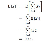
Let X be the random variable for the number of times we hire a new office assistant.
Define indicator random variables X1, X2, ... Xn where Xi = I{candidate i is hired}.
We will rely on these properties:
We need to compute Pr{candidate i is hired}:
By Lemma 1, E[Xi] = 1/i, a fact that lets us compute E[X]:
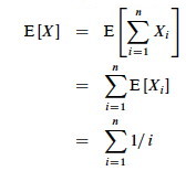
The sum is a harmonic series. From formula A7 in appendix A, the nth
harmonic number is:
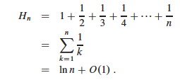
Thus, the expected hiring cost is O(ch ln n), much better than worst case O(chn)! (ln is the natural log. Formula 3.15 of the text can be used to show that ln n = O(lg n.)
We will see this kind of analysis repeatedly. Its strengths are that it lets us count in ways for which we have probabilities (compare to C.37), and that it works even when there are dependencies between variables.

Above, we had to assume a distribution of inputs, but we may not have control over inputs.
An "adversary" can always mess up our assumptions by giving us worst case inputs. (This can be a fictional adversary in making analytic arguments, or it can be a real one ...)
Randomized algorithms foil the adversary by imposing a distribution of inputs.
The modifiation to HIRE-ASSISTANT is trivial: add a line at the beginning that randomizes the list of candidates.
Having done so, the above analysis applies to give us expected value rather than average case.
What is the relationship/difference between probabilistic analysis and randomized algorithms?
There are different ways to randomize algorithms. One way is to randomize the ordering of the input before we apply the original algorithm (as was suggested for HIRE-ASSISTANT above). A procedure for randomizing an array:
  Randomize-In-Place(A)
  1  n = A.length
  2  for i = 1 to n
  3      swap A[i] with A[Random(i,n)]
The text offers a proof that this produces a uniform random permutation. It obviously runs in O(n) time.
Another approach to randomization is to randomize choices made within the algorithm.

We expect good average case behavior if all input permutations are equally likely, but what if it is not?
To get better performance on sorted or nearly sorted data -- and to foil our adversary! -- we can randomize the algorithm to get the same effect as if the input data were random.
Instead of explicitly permuting the input data (which is expensive), randomization can be accomplished trivially by random sampling of one of the array elements as the pivot.
If we swap the selected item with the last element, the existing PARTITION procedure applies:


Now, even an already sorted array will give us average behavior.
Curses! Foiled again!
The analysis assumes that all elements are unique, but with some work can be generalized to remove this assumption (Problem 7-2 in the text).
The previous analysis was pretty convincing, but was based on an assumption about the worst case. This analysis proves that our selection of the worst case was correct, and also shows something interesting: we can solve a recurrence relation with a "max" term in it!
PARTITION produces two subproblems, totaling size n-1. Suppose the partition takes place at index q. The recurrence for the worst case always selects the maximum cost among all possible ways of splitting the array (i.e., it always picks the worst possible q):

Based on the informal analysis, we guess T(n) ≤ cn2 for some c. Substitute this guess into the recurrence:
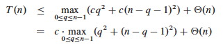
The maximum value of q2 + (n - q - 1)2 occurs when q is either 0 or n-1 (the second derivative is positive), and has value (n - 1)2 in either case:

Substituting this back into the reucrrence:

We can pick c so that c(2n - 1) dominates Θ(n). Therefore, the worst case running time is O(n2).
One can also show that the recurrence is Ω(n2), so worst case is Θ(n2).
With a randomized algorithm, expected case analysis is much more informative than worst-case analysis. Why?
This analysis nicely demonstrates the use of indicator variables and two useful strategies.
The dominant cost of the algorithm is partitioning. PARTITION removes the pivot element from future consideration, so is called at most n times.
QUICKSORT recurses on the partitions. The amount of work in each call is a constant plus the work done in the for loop. We can count the number of executions of the for loop by counting the number of comparisons performed in the loop.
Rather than counting the number of comparisons in each call to QUICKSORT, it is easier to derive a bound on the number of comparisons across the entire execution.
This is an example of a strategy that is often useful: if it is hard to count one way (e.g., "locally"), then count another way (e.g., "globally").
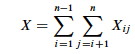
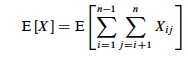
Let X be the total number of comparisons in all calls to PARTITION. The total work done over the entire execution is O(n + X), since QUICKSORT does constant work setting up n calls to PARTITION, and the work in PARTITION is proportional to X. But what is X?
For ease of analysis,
We want to count the number of comparisons. Each pair of elements is compared at most once, because elements are compared only to the pivot element and then the pivot element is never in any later call to PARTITION.
Indicator variables can be used to count the comparisons. (Recall that we are counting across all calls, not just during one partition.)
Let Xij = I{ zi is compared to zj }
Since each pair is compared at most once, the total number of comparisons is:

Taking the expectation of both sides, using linearity of expectation, and applying Lemma 5.1 (which relates expected values to probabilities):


What's the probability of comparing zi to zj?
Here we apply another useful strategy: if it's hard to determine when something happens, think about when it does not happen.
Elements (keys) in separate partitions will not be compared. If we have done two comparisons among three elements and find that zi < x <zj, we do not need to compare zi to zj (no further information is gained), and QUICKSORT makes sure we do not by putting zi and zj in different partitions.
On the other hand, if either zi or zj is chosen as the pivot before any other element in Zij, then that element (as the pivot) will be compared to all of the elements of Zij except itself.
Therefore (using the fact that these are mutually exclusive events):

We can now substitute this probability into the analyis of E[X] above and continue it:

This is solved by applying equation A.7 for harmonic series, which we can match by substituting k = j - i and shifting the summation indices down i:

We can get rid of that pesky "+ 1" in the denominator by dropping it and switching to inequality (after all, this is an upper bound analysis), and now A7 (shown in box) applies:


Above we used the fact that logs of different bases (e.g., ln n and lg n) grow the same asymptotically.
To recap, we started by noting that the total cost is O(n + X) where X is the number of comparisons, and we have just shown that X = O(n lg n).
Therefore, the average running time of QUICKSORT on uniformly distributed permutations (random data) and the expected running time of randomized QUICKSORT are both O(n + n lg n) = O(n lg n).
This is the same growth rate as merge sort and heap sort. Empirical studies show quicksort to be a very efficient sort in practice (better than the other n lg n sorts) whenever data is not already ordered. (When it is nearly ordered, such as only one item being out of order, insertion sort is a good choice.)
Here is another example of probabilistic analysis. This is Exercise 5.2-5 page 122, for which there is a publicly posted solution. This example shows the great utility of random variables.
Let A[1.. n] be an array of n distinct numbers. If i < j and A[i] > A[j], then the pair (i, j) is called an inversion of A (they are "out of order" with respect to each other). Suppose that the elements of A form a uniform random permutation of ⟨1, 2, ... n⟩.
We want to find the expected number of inversions. This has obvious applications to analysis of sorting algorithms, as it is a measure of how much a sequence is "out of order". In fact, each iteration of the while loop in insertion sort corresponds to the elimination of one inversion (see the posted solution to problem 2-4c).
If we had to count in terms of whole permutations, figuring out how many permutations had 0 inversions, how many had 1, ... etc. (sound familiar? :), that would be a real pain, as there are n! permutations of n items. Can indicator random variables save us this pain by letting us count something easier?
We will count the number of inversions directly, without worrying about what permutations they occur in:
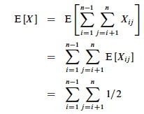
Let Xij, i < j, be an indicator random variable for the event where A[i] > A[j] (they are inverted).
More precisely, define: Xij= I{A[i] > A[j]} for 1 ≤ i < j ≤ n.
Pr{Xij = 1} = 1/2 because given two distinct random numbers the probability that the first is bigger than the second is 1/2. (We don't care where they are in a permutation; just that we can easily identify the probabililty that they are out of order. Brilliant in its simplicity!)
By Lemma 1, E[Xij] = 1/2, and now we are ready to count.
Let X be the random variable denoting the total number of inverted pairs in the array. X is the
sum of all Xij that meet the constraint 1 ≤ i <
j ≤ n:
We want the expected number of inverted pairs, so take the expectation of both sides:
Using linearity of expectation, we can simplify this far:
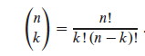
The fact that our nested summation is choosing 2 things out of n lets us write this
as:

We can use formula C.2 from the appendix:
In screencast 5A I show how to simplify this to (n(n−1))/2, resulting in:
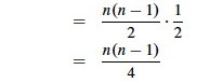
Therefore the expected number of inverted pairs is n(n − 1)/4, or O(n2).