We have been studying sorting algorithms in which the only operation that is used to gain information is pairwise comparisons between elements. So far, we have not found a sorting algorithm that runs faster than O(n lg n) time.
It turns out it is not possible to give a better guarantee than O(n lg n) in a comparison-based sorting algorithm.
The proof is an example of a different level of analysis: of all possible algorithms of a given type for a problem, rather than particular algorithms ... pretty powerful.
A decision tree abstracts the structure of a comparison sort. A given tree represents the comparisons made by a specific sorting algorithm on inputs of a given size. Everything else is abstracted, and we count only comparisons.
For example, here is a decision tree for insertion sort on 3 elements.
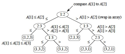
Each internal node represents a branch in the algorithm based on the information it determines by comparing between elements indexed by their original positions. For example, at the nodes labeled "2:3" we are comparing the item that was originally at position 2 with the item originally at position 3, although they may now be in different positions.
Leaves represent permutations that result. For example, "⟨2,3,1⟩" is the permutation where the first element in the input was the largest and the third element was the second largest.
This is just an example of one tree for one sorting algorithm on 3 elements. Any given comparison sort has one tree for each n. The tree models all possible execution traces for that algorithm on that input size: a path from the root to a leaf is one computation.
We don't have to know the specific structure of the trees to do the following proof. We don't even have to specify the algorithm(s): the proof works for any algorithm that sorts by comparing pairs of keys. We don't need to know what these comparisons are. Here is why:
We get our result by showing that the decision tree on the input of size n must have height at least Ω(n lg n), i.e., will have a path from the root to some leaf of length at least Ω(n lg n). This will be the lower bound on the running time of any comparison-based sorting algorithm.
h ≥ lg(n/e)n
= n lg(n/e)
= n lg n - n lg e
= Ω (n lg n).
Thus, the height of a decision tree that permutes n elements to all possible permutations cannot be less than n lg n.
A path from the leaf to the root in the decision tree corresponds to a sequence of comparisons, so there will always be some input that requires at least Ω(n lg n) comparisions in any comparision based sort.
There may be some specific paths from the root to a leaf that are shorter. For example, when insertion sort is given sorted data it follows an O(n) path. But to give an o(n lg n) guarantee (i.e, strictly better than O(n lg n)), one must show that all paths are shorter than O(n lg n), or that the tree height is o(n lg n) and we have just shown that this is impossible since it is Ω(n lg n).
Sometimes, if we know something about the structure of the data, it is possible to sort it without comparing elements to each other. Since we do not need to do comparisons, we can sort data faster than the Ω(n lg n) lower bound presented above. How is this possible? Answer.
Typically these algorithms work by using information about the keys themselves to put them "in their place" without comparisons. Here we describe several algorithms that are able to sort data in O(n) time.
Assumes (requires) that keys to be sorted are integers in {0, 1, ... k}.
For each element in the input, determines how many elements are less than that input.
Then we can place the element directly in a position that leaves room for the elements that come after it.
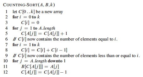
An example ...
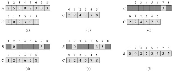
Counting sort is a stable sort, meaning that two elements that are equal under their key will stay in the same order as they were in the original sequence. This is a useful property ...
Counting sort requires Θ(n + k). If k<n, counting sort runs in Θ(n) time.

Using a stable sort like counting sort, we can sort from the least to the most significant digit:
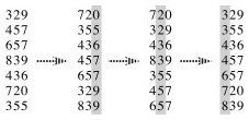
This is how punched card sorters used to work.
The code is trivial, but requires a stable sort and only works on n d-digit numbers in which each digit can take up to k possible values:

If the stable sort used is Θ(n + k) time (like counting sort) then RADIX-SORT is Θ(d(n + k)) time.
Bucket Sort maps the keys to the interval [0, 1), placing each of the n input elements into one of n buckets. If there are collisions, chaining (linked lists) are used.
Next, the algorithm sorts each chain using any known sorting algorithm, e.g. insertion sort.
Finally, the algorithm outputs the contents of each bucket in order of the buckets, by contactenating the chains.
The algorithm assumes that the input is from a uniform distribution, i.e., each key is equally likely to fall into either bucket. Then each chain is expected to contain a constant number of items and, therefore, the sorting of each chain is expected to take O(1) time.
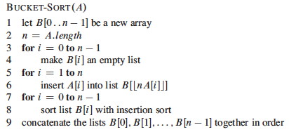
The numbers in the input array A are thrown into the buckets in B according to their magnitude. For example, 0.78 is put into bucket 7, which is for keys 0.7 ≤ k < 0.8. Later on, 0.72 maps to the same bucket: like chaining in hash tables, we "push" it onto the beginning of the linked list.
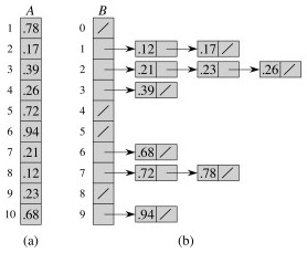
At the end, we sort the lists (B shows the lists after they are sorted; otherwise we would have 0.23, 0.21, 0.26) and then copy the values from the lists back into an array.
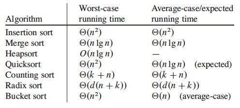
You can also compare some of the sorting algorithms with these animations (set to 50 elements): http://www.sorting-algorithms.com/. Do the algorithms make more sense now?