ICS 311 #12B: Dynamic Programming (cont.)

Outline

1. More examples of Dynamic Programming: Longest Common Subsequence
2. Summary and Comments on Optimal Substructure

Readings and Screencasts

• Read CLRS 14.4-14.5. The focus is on the problem solving strategy: Read the examples primarily to understand the Dynamic Programming strategy rather than to memorize the specifics of each problem (although you might be asked to trace through some of the algorithms).
• Screencasts 12B (5:00-end), 12C, 12D (6:17-end) (also in Laulima)

Another Example: Longest Common Subsequence

A subsequence of sequence S leaves out zero or more elements but preserves order.

Z is a common subsequence of X and Y if Z is a subsequence of both X and Y.
Z is a longest common subsequence if it is a subsequence of maximal length.

The LCS Problem

Given two sequences X = ⟨ x₁, ..., x_m ⟩ and Y = ⟨ y₁, ..., y_n ⟩, find a subsequence common to both whose length is longest. Solutions to this problem have applications to DNA analysis in bioinformatics. The analysis of optimal substructure is elegant.

Examples

Brute Force Algorithm

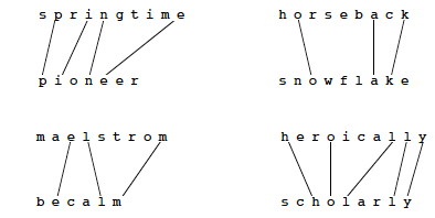
For every subsequence of X = ⟨ x₁, ..., x_m ⟩, check whether it is a subsequence of Y = ⟨ y₁, ..., y_n ⟩, and record it if it is longer than the longest previously found.

• There are 2^m subsequences of X to check.
• For each subsequence, scan Y for the first letter. From there scan for the second letter, etc., up to the n letters of Y.
• Therefore, Θ(n2^m).

This involves a lot of redundant work.

• If a subsequence Z of X fails to match Y, then any subsequence having Z as a prefix will also fail.
• If a subsequence Z of X matches Y, then there is no need to check prefixes of Z.

Many problems to which dynamic programming applies have exponential brute force solutions that can be improved on by exploiting redundancy in subproblem solutions.

Step 1. Optimal Substructure of LCS

The first step is to characterize the structure of an optimal solution, hopefully to show it exhibits optiomal stubstructure.

Often when solving a problem we start with what is known and then figure out how to contruct a solution. The optimal substructure analysis takes the reverse strategy: assume you have found an optional solution (Z below) and figure out what you must have done to get it!

Notation:

• X_i = prefix ⟨ x₁, ..., x_i ⟩
• Y_i = prefix ⟨ y₁, ..., y_i ⟩

Theorem: Let Z = ⟨ z₁, ..., z_k ⟩ be any LCS of X = ⟨ x₁, ..., x_m ⟩ and Y = ⟨ y₁, ..., y_n ⟩. Then

1. If x_m = y_n, then z_k = x_m = y_n, and Z_k-1 is an LCS of X_m-1 and Y_n-1.
2. If x_m ≠ y_n, then z_k ≠ x_m ⇒ Z is an LCS of X_m-1 and Y.
3. If x_m ≠ y_n, then z_k ≠ y_n ⇒ Z is an LCS of X and Y_n-1.

Sketch of proofs:

(1) can be proven by contradiction: if the last characters of X and Y are not included in Z, then a longer LCS can be constructed by adding this character to Z, a contradiction.

(2) and (3) have symmetric proofs: Suppose there exists a subsequence W of X_m-1 and Y (or of X and Y_n-1) with length > k. Then W is a common subsequence of X and Y, contradicting Z being an LCS.

Therefore, an LCS of two sequences contains as prefix an LCS of prefixes of the sequences. We can now use this fact construct a recursive formula for the value of an LCS.

Step 2. Recursive Formulation of Value of LCS

Let c[i, j] be the length of the LCS of prefixes X_i and Y_j. The above recursive substructure leads to the definition of c:

We want to find c[m, n].

Step 3. Compute Value of Optimal Solution to LCS

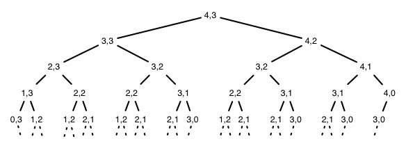
A recursive algorithm based on this formulation would have lots of repeated subproblems, for example, on strings of length 4 and 3:

Dynamic programming avoids the redundant computations by storing the results in a table. We use c[i,j] for the length of the LCS of prefixes X_i and Y_j (hence it must start at 0). (b is part of the third step and is explained next section.)

Try to find the correspondence betweeen the code below and the recursive definition shown in the box above.

This is a bottom-up solution: Indices i and j increase through the loops, and references to c always involve either i-1 or j-1, so the needed subproblems have already been computed.

It is clearly Θ(mn); much better than Θ(n2^m)!

Step 4. Construct an Optimal Solution to LCS

In the process of computing the value of the optimal solution we can also record the choices that led to this solution. Step 4 is to add this latter record of choices and a way of recovering the optimal solution at the end.

Table b[i, j] is updated above to remember whether each entry is

• a common substring of X_i-1 and Y_j-1 (diagonal arrow), in which case the common character x_i = y_j is included in the LCS;
• a common substring of X_i-1 and Y (↑); or
• a common substring of X and Y_j-1 (←).

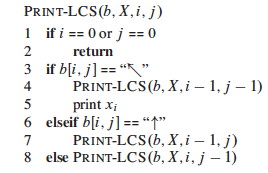
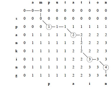
We reconstruct the path by calling Print-LCS(b, X, n, m) and following the arrows, printing out characters of X that correspond to the diagonal arrows (a Θ(n + m) traversal from the lower right of the matrix to the origin):

Example of LCS

What do "spanking" and "amputation" have in common?

Another Application

Another application of Dynamic Programming is covered in the Cormen et al. textbook (Section 14.4). I briefly describe the problem here, but you are responsible for reading the details of the solution in the book. Many more applications are listed in the problems at the end of the Chapter 14.

Optimal Binary Search Tree

We saw in Topic 8 that an unfortunate order of insertions of keys into a binary search tree (BST) can result in poor performance (e.g., linear in n). If we know all the keys in advance and also the probability that they will be searched, we can optimize the construction of the BST to minimize search time in the aggregate over a series of queries. An example application is when we want to construct a dictionary from a set of terms that are known in advance along with their frequency in the language. The reader need only try problem 14.5-2 from the Cormen et al. text (manual simulation of the algorithm) to appreciate why we want to leave this tedium to computers!

Further Observations Concerning Optimal Substructure

To use dynamic programming, we must show that any optimal solution involves making a choice that leaves one or more subproblems to solve, and the solutions to the subproblems used within the optimal solution must themselves be optimal.

The optimal choice is not known before solving the subproblems

We may not know what that first choice is. Consequently:

• To show that there is optimal substructure, we suppose that the choice has been made, and show that the subproblems that result must also be solved optimally. This argument is often made using a cut-and-paste proof by contradiction.
• Then when writing the code, we must ensure that enough potential choices and hence their supbproblems are considered that we find the optimal first choice. This usually shows up as iteration in which we find the maximum or minimum according to some objective function across all choices.

Optimal substructure varies across problem domains:

How many subproblems are used in an optimal solution may vary:

• Rod Cutting: 1 subproblem (of size n - i)
• LCS: 1 subproblem (LCS of the prefix sequence(s).)
• Optimal BST: 2 subproblems (given k_r has been chosen as the root, k_i ..., k_r-1 and k_r+1 ..., k_j)

How many choices in determining which subproblem(s) to use may vary:

• Rod cutting: n choices (for each value of i)
• LCS: Either 1 choice (if x_i = y_j, take LCS of X_i-1 and Y_j-1), or 2 choices (if x_i ≠ y_j, check both LCS of X_i-1 and Y, and LCS of X and Y_j-1)
• Optimal BST: j - i + 1 choices for the root k_r in k_i ..., k_j: see text.

Informally, running time depends on (# of subproblems overall) x (# of choices).

• Rod Cutting: Θ(n) subproblems overall, ≤ n choices for each ⇒ O(n²) running time.
• LCS: Θ(mn) subproblems overall; ≤ 2 choices for each ⇒ O(mn) running time.
• Optimal BST: Θ(n²) subproblems overall; O(n) choices for each ⇒ O(n³) running time.

(We'll have a better understanding of "overall" when we cover amortized analysis.)

Not all optimization problems have optimal substructure

When we study graphs, we'll see that finding the shortest path between two vertices in a graph has optimal substructure: if p = p₁ + p₂ is a shortest path between u and v then p₁ must be a shortest path between u and w (etc.). Proof by cut and paste.

But finding the longest simple path (the longest path not repeating any edges) between two vertices is not likely to have optimal substructure.

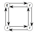
For example, q → s → t → r is longest simple path from q to r, and r → q → s → t is longest simple path from r to t, but the composed path is not even legal: the criterion of simplicity is violated.

Dynamic programming requires overlapping yet independently solveable subproblems.

Longest simple path is NP-complete, a topic we will cover at the end of the semester, so is unlikely to have any efficient solution.

Dynamic programming uses optimal substructure bottom up

Although we wrote the code both ways, in terms of the order in which solutions are found, dynamic programming first finds optimal solutions to subproblems and then choses which to use in an optimal solution to the problem. It applies when one cannot make the top level choice until subproblem solutions are known.

In Topic 13, we'll see that greedy algorithms work top down: first make a choice that looks best, then solve the resulting subproblem. Greedy algorithms apply when one can make the top level choice without knowing how subproblems will be solved.

Summary

Dynamic Programming applies when the problem has these characteristics:

Recursive Decomposition

The problem has recursive structure: it breaks down into smaller problems of the same type. This characterisic is shared with divide and conquer, but dynamic programming is distinguished from divide and conquer by the next item.

Overlapping Subproblems

The subproblems solved by a recursive solution overlap (the same subproblems are revisited more than once). This means we can save time by preventing the redundant computations.

Optimal Substructure

Any optimal solution involves making a choice that leaves one or more subproblems to solve, and the solutions to the subproblems used within the optimal solution must themselves be optimal. This means that optimized recursive solutions can be used to construct optimized larger solutions.

Dynamic programming can be approached top-down or bottom-up:

Top-Down with memoization:

Write a recursive procedure to solve the problem, computing subproblems as needed. Each time a sub-problem is encountered, see whether you have stored it in a table, and if not, solve it and store the solution.

Bottom-Up:

Order the subproblems such that "smaller" problems are solved first, so their solutions are available in the table before "larger" problems need them. (This ordering need not be based on literal size.)

Both have the same asympotic running time. The top-down procedure has the overhead of recursion, but computes only the subproblems that are actually needed. Bottom-up is used the most in practice.

We problem solve with dynamic programming in four steps:

1. Characterize the structure of an optimal solution:
   • How are optimal solutions composed of optimal solutions to subproblems?
2. Recursively define the value of an optimal solution:
   • Write a recursive cost function that reflects the above structure
3. Compute the value of an optimal solution:
   • Write code to compute the recursive values, memoizing or solving smaller problems first to avoid redundant computation
4. Construct an optimal solution from the computed information:
   • Augment the code as needed to record the structure of the solution

Wrapup

There is an online presentation focusing on LCS at http://www.csanimated.com/animation.php?t=Dynamic_programming.

In the next Topic 13 we look at a related optimization strategy: greedy algorithms.