"Although this may seem a paradox, all exact science is dominated by the idea of approximation." − Bertrand Russell

Well, your boss understands it's a hard problem, but he still wants you to do something about it! After all, we can't abandon the lucrative iThingy market! Is there a way to configure iThingies to be "good enough" without using a huge amount of computer time delaying the orders?
There are three broad approaches to handing NP-Complete or NP-Hard problems in practice:
Let C be the cost of a solution found for a problem of size n and C* be the optimal solution for that problem.
Then we say an algorithm has an approximation ratio of ρ(n) (that's "rho") if
C/C* ≤ ρ(n) for minimization problems: the factor by which the actual solution obtained is larger than the optimal solution.
C*/C ≤ ρ(n) for maximization problems: the factor by which the optimal solution is larger than the solution obtained
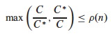
The CLRS text says both of these at once in one expression shown to the right. The ratio is never less than 1 (perfect performance).
An algorithm that has an approximation ratio of ρ(n) is called a ρ(n)-approximation algorithm.
An approximation scheme is a parameterized approximation algorithm that takes an additional input ε > 0 and for any fixed ε is a (1+ε)-approximation algorithm. (ε is how much slack you will allow away from the optimal 1-"approximation".)
An approximation scheme is a polynomial approximation scheme if for any fixed ε > 0 the scheme runs in time polynomial in input size n. (We will not be discussing approximation schemes today; just wanted you to be aware of the idea. See section 35.5)
By definition, if a problem A is NP-Complete then if we can solve A in O(f(n)) then we can solve any other problem B in NP in O(g(n)) where g(n) is polynomially related to f(n). (A polynomial time reduction of the other problems to A exists.)
So, if we have a ρ(n)-approximation algorithm for the optimization version of A, does this mean we have a ρ(n)-approximation algorithm for the optimization version of any problem B in NP? Can we just use the same polynomial time reduction, and solve A, to get a ρ(n)-approximation for B?
That would be pretty powerful! Below we show we have a 2-approximation algorithm for NP-Hard Vertex Cover: so is 2-approximation possible for the optimization version of any problem in NP? (See problem 35.1-5.)
We examine two examples in detail before summarizing other approximation strategies.
Recall that a vertex cover of an undirected graph G = (V, E) is a subset V' ⊆ V such that if (u, v) ∈ E then u ∈ V' or v ∈ V' or both (there is a vertex in V' "covering" every edge in E).
The optimization version of the Vertex Cover Problem is to find a vertex cover of minimum size in G.
We previously showed by reduction of CLIQUE to VERTEX-COVER that the corresonding decision problem is NP-Complete, so the optimization problem is NP-Hard.
Vertex Cover can be approximated by the following surprisingly simple algorithm, which iterately chooses an edge that is not covered yet and covers it:
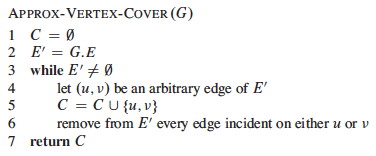
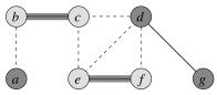
Suppose we have this input graph:
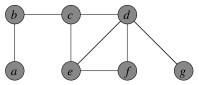
Suppose then that edge {b, c} is chosen. The two incident vertices are added to the cover and all other incident edges are removed from consideration:
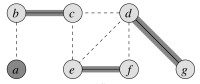
Iterating now for edges {e, f} and then {d, g}:
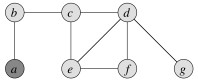
The resulting vertex cover is shown on the left and the optimal vertex on the right:
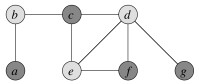
(Would the approximation bound be tighter if we always chose an edge with the highest degree vertex remaining? Let's try it on this example. Would it be tighter in general? See 35.1-3.)
How good is the approximation? We can show that the solution is within a factor of 2 of optimal.
Theorem: Approx-Vertex-Cover is a polynomial time 2-approximation algorithm for Vertex Cover.
Proof: The algorithm is correct because it loops until every edge in E has been covered.
The algorithm has O(|E|) iterations of the loop, and (using aggregate analysis, Topic 15) across all loop iterations, O(|V|) vertices are added to C. Therefore it is O(E + V), so is polynomial.
It remains to be shown that the solution is no more than twice the size of the optimal cover. We'll do so by finding a lower bound on the optimal solution C*.
Let A be the set of edges chosen in line 4 of the algorithm. Any vertex cover must cover at least one endpoint of every edge in A. No two edges in A share a vertex (see algorithm), so in order to cover A, the optimal solution C* must have at least as many vertices:
| A | ≤ | C* |
Since each execution of line 4 picks an edge for which neither endpoint is yet in C and adds these two vertices to C, then we know that
| C | = 2 | A |
Therefore:
| C | ≤ 2 | C* |
That is, |C| cannot be larger than twice the optimal, so is a 2-approximation algorithm for Vertex Cover.
This is a common strategy in approximation proofs: we don't know the size of the optimal solution, but we can set a lower bound on the optimal solution and relate the obtained solution to this lower bound.
Can you come up with an example of a graph for which Approx-Vertex-Cover always gives a suboptimal solution?
Suppose we restrict our graphs to trees. Can you give an efficient greedy algorithm that always finds an optimal vertex cover for trees in linear time?
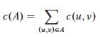
In the Traveling Salesperson Problem (TSP) we are given a complete undirected graph G = (V, E) (representing, for example, routes between cities) that has a nonnegative integer cost c(u, v) for each edge {u, v} (representing distances between cities), and must find a Hamiltonian cycle or tour with minimum cost. We define the cost of such a cycle A to be the sum of the costs of edges:
The unrestricted TSP is very hard, so we'll start by looking at a common restriction.
In many applications (e.g., Euclidean distances on two dimensional surfaces), the TSP cost function satisfies the triangle inequality:

c(u, v) ≤ c(u, w) + c(w, v), ∀ u, v, w ∈ V.
Essentially this means that it is no more costly to go directly from u to v than it would be to go between them via a third point w.
The triangle inequality TSP is still NP-Complete, but there is a 2-approximation algorithm for it. The algorithm finds a minimum spanning tree (Topic 17), and then converts this to a low cost tour:
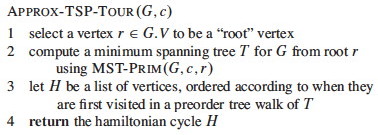
(Another MST algorithm might also work.)
Suppose we are working on the graph shown below to the left. (Vertices are placed on a grid so you can compute distances if you wish.) The MST starting with vertex a is shown to the right.
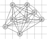
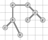
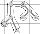
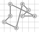
Recall from early in the semester (or ICS 241) that a preorder walk of a tree visits a vertex before visiting its children. Starting with vertex a, the preorder walk visits vertices in order a, b, c, h, d, e, f, g. This is the basis for constructing the cycle in the center (cost 19.074). The optimal solution is shown to the right (cost 14.715).
Theorem: Approx-TSP-Tour is a polynomial time 2-approximation algorithm for TSP with triangle inequality.
Proof: The algorithm is correct because it produces a Hamiltonian circuit.
The algorithm is polynomial time because the most expensive operation is MST-Prim, which can be computed in O(E lg V) (see Topic 17 notes).
For the approximation result, let T be the spanning tree found in line 2, H be the tour found and H* be an optimal tour for a given problem.
If we delete any edge from H*, we get a spanning tree that can be no cheaper than the minimum spanning tree T, because H* has one more (nonegative cost) edge than T:
c(T) ≤ c(H*)
Consider the cost of the full walk W that traverses the edges of T exactly twice starting at the root. (For our example, W is ⟨{a, b}, {b, c}, {c, b}, {b, h}, {h, b}, {b, a}, {a, d}, ... {d, a}⟩.) Since each edge in T is traversed twice in W:
c(W) = 2 c(T)
This walk W is not a tour because it visits some vertices more than once, but we can skip the redundant visits to vertices once we have visited them, producing the same tour H as in line 3. (For example, instead of ⟨{a, b}, {b, c}, {c, b}, {b, h}, ... ⟩, go direct: ⟨{a, b}, {b, c}, {c, h}, ... ⟩.)
By the triangle inequality, which says it can't cost any more to go direct between two vertices,
c(H) ≤ c(W)
Noting that H is the tour constructed by Approx-TSP-Tour, and putting all of these together:
c(H) ≤ c(W) = 2 c(T) ≤ 2 c(H*)
So, c(H) ≤ 2 c(H*), and thus Approx-TSP-Tour is a 2-approximation algorithm for TSP. (The CLRS text notes that there are even better solutions, such as a 3/2-approximation algorithm.)
Another algorithm that is a 2-approximation on the triangle inequality TSP is the closest point heuristic, in which one starts with a trivial cycle including a single arbitrarily chosen vertex, and at each iteration adds the next closest vertex not on the cycle until the cycle is complete.
Above we got our results using a restriction on the TSP. Unfortunately, the general problem is harder ...
Theorem: If P ≠ NP, then for any constant ρ ≥ 1 there is no polynomial time approximation algorithm with ratio ρ for the general TSP.
The proof by contradiction shows that if there were such an approximation one can solve instances of Hamiltonian Cycle in polynomial time. Since Hamiltonian Cycle is NP-Complete, then P = NP. The proof uses a reduction similar to that used in Topic 24, where edges for TSP graph G' are given unit cost only if the corresponding edge is in the edge-set E for the Hamiltonian Cycle problem graph G:
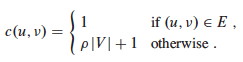
For any ρ(n) ≥ 1, a TSP approximation algorithm will choose the edges of cost 1 in G' (because to include even one edge not in E would exceed the approximation ratio), thereby finding a Hamiltonian Cycle in G if such a cycle exists. (See text for details.)
We have just seen that even within NP, some problems are harder than others in terms of whether they allow approximations.
The proof technique of reduction to NP-Complete problems has been used to organize the class NPC into problems that can be polynomially approximated and those that cannot under the assumption that P ≠ NP. Further discussion can be found in Garey and Johnson (1979).
You can probably guess that the answer to the question I raised in the beginning concerning transfer of ρ(n)-approximation across problem reductions is negative, but why would that be the case? Why aren't approximation properties carried across problem reductions?
Various reusable strategies for approximations have been found, two of which we review briefly here.
Sometimes it is possible to obtain an adequate approximation ratio with a greedy approach.
Here is a brief example, covered in more detail in CLRS 3.5.3.Suppose we are given a finite set of elements X, and a "family" or set of subsets F such that every element of X belongs to at least one set in F. That is, F covers X. But do we need all of the subsets in F to cover X?
The SET-COVER problem is to find a minimum subset of F (minimum number of subsets) that cover all of X (the union of the subsets is X).
VERTEX-COVER can be reduced to SET-COVER, so the latter is NP-Complete.
This problem has applications to finding the minimum resources needed for a situation, such as the minumum number of people (represented by the subsets of F) with the skills (represented by members of X) needed to carry out a task or solve a problem.
A greedy approximation algorithm for SET-COVER is as follows:
  Greedy-Set-Cover (X, F)
  1  U = X                      // the remaining elements we need to cover
  2  C = {}                     // the subset of F we have chosen
  3  while U != {}
  4      select an S ∈ F that maximizes |S ∩ U|
  5      U = U − S             // we are now covering the elements of S ...
  6      C = C ∪ {S}           // ... by adding S to our chosen subsets
  7  return C
CLRS show that Greedy-Set-Cover can be implemented in polynomial time, and furthermore that it is an ρ(n)-approximation algorithm, where ρ(n) is related to the size of the maximum set in F, max{|S| : S ∈ F}, a small constant in some applications.
You can see CLRS for details: The main point here is to make you aware that sometimes greedy algorithms work as approximation algorithms.
The approximation ratio ρ(n) of a randomized algorithm is based on its expected cost C. Otherwise the definition is the same.
A randomized algorithm that achieves an expected cost within a factor ρ(n) of the optimal cost C* is called a randomized ρ(n)-approximation algorithm.
Recall that 3-CNF-SAT (Topic 24) asks whether a boolean formula in 3-conjunctive normal form (3-CNF) is satisfiable by an assignment of truth values to the variables.
The Max-3-CNF variation is an optimization problem that seeks to maximize the number of conjunctive clauses evaluating to 1. We assume that no clause contains both a variable and its negation.
Amazingly, a purely random solution is expected to be pretty good:
Theorem: The randomized algorithm that independently sets each variable of MAX-3-CNF to 1 with probability 1/2 and to 0 with probabilty 1/2 is a randomized 8/7-approximation algorithm.
Proof: Given a MAX-3-CNF instance with n variables x1 ... xn and m clauses, set each variable randomly to either 0 or 1 with probability 1/2 in each case. Define the indicator random variable (Topic 5):
Yi = I{clause i is satisfied}.
A clause is only unsatisfied if all three literals are 0, so Pr{clause i is not satisfied} = (1/2)3 = 1/8. Thus, Pr{clause i is satisfied} = 7/8. By an important lemma from Topic 5, E[Yi] = 7/8.
Let Y = Σ Y1 ... Ym be the number of clauses satisified overall. Then:
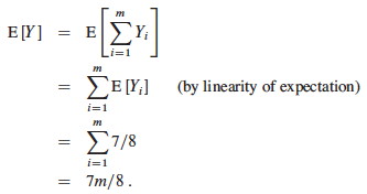
Since m is the upper bound C* on the number of satisfied clauses, the approximation ratio C* / C is
m / (7m/8) = 8/7.
The restriction on a variable and its negation can be lifted. This is just an example: randomization can be applied to many different problems − but don't always expect it to work out so well!
It is worth reading the other examples in the text.
Section 35.3 shows how the Set Covering Problem, which has many applications, can be approximated using a simple greedy algorithm with a logarithmic approximation ratio.
Section 35.5 uses the Subset Sum problem to show how an exponential but optimal algorithm can be transformed into a fully polynomial time approximation scheme, meaning that we can give the algorithm a parameter specifying the desired approximation ratio.
Many more examples are suggested in the problem set for the chapter.
Faced with an NP Hard optimization problem, your options include: