N otes on Chapter 4
pp 27 - 37 of your lab book

Please read the section on error analysis in my web page.  We will be covering those notes.  The error analysis page has notes on: 1) The definition of an error,  2) Random and systematic errors, 3) propagation of uncertainties, and 4) statistical analysis of uncertainties.  These notes can be found at:

http://www2.hawaii.edu/~jmcfatri/labs/erroranalysis.html

In everyday language, accuracy and precision are interchangeable terms.  Sometimes even I get them mixed up when I talk. However, in physics they mean two entirely different things and you should try to keep them separate as much as possible.

• Accuracy is the "closeness" to the known or actual result. This is what you are discussing in your Compare To Known section
• Precision is the amount of confidence you have in the result. This is what you are discussing when you talk about errors or uncertainty.

You can have an accurate measurement that is not precise.  Example: You could say that a car is going 50 +/- 50 mph. The actual speed is within this range, so you have an accurate measurement.  However, you do not have very much precision in this measurement.

You can have a precise measurement that is not accurate.  Example: You could measure the speed of the car was 54.003 +/- 0.001 mph, which is a very precise measurement.  However, if you found that the car could only reach speeds of 25 mph, you would know that your measurement was not accurate.

The Gaussian Distribution
A Gaussian distribution is any function of the form f(u) = Ae^{-u 2} . A plot of f(u) vs. u shows a familiar bell curve.

 

When we make a histogram of a measured quantity, we often find that our result, after many measurements, looks like a Gaussian distribution. (A histogram is a plot of the number of times you saw the value versus the value itself.)  This is an indication of random errors.  Random errors are not completely random in their distribution.  If you repeatedly measured the length of a pen of actual length 18.2 cm, you would expect that most of your data values would be close to 18.2 cm, and very few would be out at 18.4 cm. You would not expect to get 18.4 cm as often as you get 18.2 cm, certainly! That is exactly what a Gaussian distribution says.  It says there is more probability of getting some data points than others.

• Can you see from this argument that the wider the Gaussian, the less precision you have in your measurement?

 If the Gaussian is very narrow, that means that you have a high probability of getting close to the average (peak value).  If the Gaussian is very wide, then you have about equal probability of getting the peak value as a value far from the peak.

Thus, Gaussian distributions are a good way of characterizing data with random uncertainties. The width of the Gaussian is now defined to be the uncertainty in the measurement. It is also the standard deviation of the measurement! The width of a Gaussian is defined to be the points of inflection on the curve, or where you have 68% of finding the value.

Rewriting the formula above in terms of Amplitude (A),  and width (w), and if u = v/w, then I have f(v) = Ae^-(v/w)2.

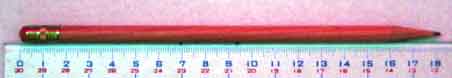
Now I will pass a pencil around the room.  Measure the length of the pencil in cm to as great a precision as you can achieve.  I will come by and write down your values. (Do NOT discuss your value with your neighbor).

I will write down the results on the board.  In the space below, make a histogram of our measurements.


















The Normalized Gaussian Distribution
We are talking about probabilities of finding a particular value and we are defining the width of a Gaussian in terms of probability. It makes sense then, to plot our data not as a histogram, but as a plot of the fraction of times we saw the value versus the value itself. (Anotherwords, take your histogram and divide all your points by the total number of times you made the measurement.)  If you do this, you will find that this new distribution is still a Gaussian!  The difference is that now the area under the curve represents a probability.  It is the probability of finding the next measurement in the range over which you are taking the area.

If you do this, you are normalizing your Gaussian. The Gaussian is then called a normalized Gaussian distribution. A normalized Gaussian distribution has total area equal to 1 (anotherwords, the probability of finding a value between -infinity and +infinity is 100%). A normalized Gaussian distribution which has a width (w), total number of measurements (N), and peak value (p), is given by:

 

 
Now let's normalize our values. In the space below, plot the fraction of times we saw each value versus the value itself.

Assignments: