Lab #3b: Numerically Integrating the Ultra-high Energy Cosmic ray
spectrum
1. Introduction: Ultra-high energy cosmic rays (UHECR)
For more than 40 years, particle detectors have been
recording interactions of what are apparently single subatomic
particles with almost unbelievable energies of as much as 3 X 10²⁰
eV, nearly 50 Joules (1 eV = 1.6 X 10⁻¹⁹ J). These particles
are known generally as cosmic
rays, and these super-energy varieties are called the Ultra-high Energy
Cosmic Rays (UHECR). If these are single hydrogen nuclei (protons) as
is widely believed, then they have Lorentz relativistic gamma-factors
of more than 1011. Since the highest energy that we can
produce with earth-based proton accelerators is about 1012
eV (gamma factor of 103 ) which is about 100 Million times
less energy, there is intense interest to determine how nature makes
such particles, and how they manage to propagate in the universe.
Standard particle physics theories say that they should be degraded in
energy very quickly in intergalactic space through collisions with the
cosmic microwave background radiation, which appears boosted to
gamma-ray energies in the Lorentz center-of-momentum frame. However,
such particles seem to somehow evade this process, since we still see
them at energies greater than 5 x 10¹⁹ eV where they should
be completely absorbed in space.
Measurements of the flux of particles arriving at earth have
been made over the last four decades, and here is one such result, from
a detector in Utah called the High Resolution Fly's Eye:
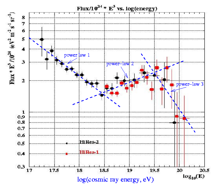
Figure
1: Ultra-high energy cosmic ray spectrum
This is a complicated graph, with data in black and red, but with each
data point multiplied by the cube of its energy along the x-axis,
because the graph is otherwise so steeply falling that it is difficult
to view. The cosmic-ray fluxes (once the energy3 is divided
out) have units of particles per m2 per steradian per
second per eV.
2. Power law energy spectra
A power-law energy
spectrum is a function of the form
F(E) = A0
(E/E0)-p
(1)
where E is the particle energy, and A0 , E0
and p are parameters that determine the shape. An energy spectrum in this case is
defined as a function which gives the number of particles observed as a
function of their energy. For example, a glass prism held up to the sun
produces a rainbow "spectrum" of light, and if we had a way to measure
the intensity of each color, we would have a spectrum of the
sun's photon intensity as a function of wavelength (remember for
photons the wavelength is inversely proportional to energy, E =
[Planck's constant]*[speed of light]/[wavelength] ).
The energy spectrum we consider here is called a power-law because it depends on an
exponential power of the independent variable (energy E in this case),
thus the general form is f(x) = xp.
If we take the logarithm
of the spectrum equation (1) above:
log(F(E)) = log(A0) -
p*log(E) + p*log(E0)
= -p*log(E) + [ log(A0) - p* log(E0)
]
(2)
then we get an equation which has the form y = m*x +
b, the equation of a line with the following substitutions:
y =
log(F(E)), m = -p, x = log(E)
and b = [ log(A0) - p*
log(E0) ].
Because of this linear relationship in the logarithm, power-law
functions are nice for fitting and display, and have a suprising degree
of relevance for many physical processes in particle acceleration. The
functions themselves (not necessarily as a logarithm) can also be
integrated analytically.
For the spectrum shown in Fig. 1 above, the three sections of power-law
shown are not certain to be correct, but they fit the data reasonably
well, and have
some physics basis, since natural particle accelerators that we know of
often produce power-law behavior in their outputs.
In this case "Power-law 1" represents the underlying energy
spectrum
of accelerated high energy protons trapped within our galaxy by
magnetic fields. At
around 3e18 eV (shorthand for 3 X 10¹⁸ eV), such particles
have enough energy that they can overcome magnetic confinement, and can
escape
not only from our galaxy but also from other nearby galaxies, and an
enhancement is expected as new cosmic rays enter in from the outside,
leading to "Power-law 2."
Finally even the outside cosmic rays start to
get absorbed in intergalactic space due to interactions with the
microwave background and this leads to a steepening of the spectrum at
"Power law 3," eventually leading to a cutoff in the spectrum, known as
the Greisen-Zatsepin-Kuzmin (GZK) cutoff. This cutoff is not yet
clearly observed, but is expected to terminate the spectrum shown. It
is due to the fact that the high energy protons, once they get to
energiies of about 1020 eV, begin to see the Big Bang
microwave photons as gamma-rays in their own center-of-momentum
reference frame (remember Einstein's special relativity means that
these UHECR protons have their own frame of reference relative to
everything else--to them, galaxies are zipping by at the speed of
light). Protons encountering a stream of gamma-rays eventually get
blasted apart, and so UHECR protons cannot go very far in intergalactic
space.
The energy spectra above in Fig. 1 are going to become the functions we
will numerically integrate. First we need to express them in analytic
form.
Here are the actual power law functions including parameters, units,
and limits:
Power-law 1:
F1(E) = 5 X 10-27
( E/1017 ) -3.35 m-2
s-1 sr-1 eV-1 ,
where E1a= 1017 eV <= E
<= E1b=3 X 10¹⁸
eV
Power-law 2:
F2(E) = 5.5 X 10⁻³²
( E/(3 X
1018 ) ) -2.79 m-2
s-1
sr-1 eV-1 ,
where E2a=3 X 10¹⁸
eV <=
E <= E2b=2.5 X 10¹⁹
eV
Power-law 3:
F3(E) = 1.5 X 10⁻³⁴
( E/(2.5 X
1019 ) ) -3.49
m-2
s-1 sr-1 eV-1 ,
where E3a=2.5 X
1019 <= E
<= E3b=1021eV
The units here are particles per square meter per second per steradian
per electron volt (of energy). If you do not recall how to work with
solid angle (measured in sr = ster =
steradians) you can review it at this
(wikipedia) site. Solid angle can be though of as the measure of
the collection of all possible arrival directions for the particles
over the sky. It is the "size" measured in units of radians2
(this is dimensionally what steradians look like) of that part of the
sky over which the intensity originates. You can also think of it as
square degrees if that helps. For example, the sun, which is about 1/2
a degree in angular diameter, has a solid angle of pi*(0.5)2
/4 = 0.196 square degrees. There are 3282.8 square degrees in a
steradian, and the sun thus has a solid angle of about 6 X 10⁻⁵
steradians.
The data in the plot above is given (in Microsoft Excel format) in the
file UHECRspec.csv. Take a look at
this data file to make sure you understand what is inside of it. A plot
file, uhecr.plt, is also given, to plot
these data and the functions above in gnuplot. Try manipulating uhecr.plt to create a graph with the E3
scaling given above, by multiplying the functions and the y-axis data
by E3 (you will need to use special construction
for the arguments of the plot command--see previous plot files for
this). This type of scaling distorts the data, but in a way that
accentuates the differences in the three energy regimes of the plot.
To numerically integrate them you now construct piecewise
definite integrals for each segment of energy.

where m=1, 2, 3 for the different power-law pieces. These are each
numerically integrated.
Then the total flux of particles becomes
Itotal = I1
+ I2 + I3
which gives particles per square meter per second per steradian.
3. Assignment, part C:
Starting with the plot file above, create three separate log-log plots
of the three different energy ranges of the data given above, including
the functional fits given above. Change the ranges so that only the
section of interest is plotted. Change the functions so that the
endpoints are not truncated to zero out-of-range (that is, remove the
conditional statement for the functions). Include also the summary plot
given in the plotfile above.
Using your new numerical integration skills from part A & B
of Lab #3a, write a C program to integrate numerically the three
power law spectra above to determine the number of particles detected
per year over a square detector with size 10 km on a side (100 square
km), which can accept particles over 1 steradian of solid angle. Give
total integrated rates (particles per year) for minimum energies of 1017
eV, 1018
eV, 1019 eV, and 1020 eV in
an html table.
Note that this will require adjusting
the lower limits of some of you
numerical integrals above to match these round values. You must also do
the numerical integrals with the linearized (not logarithmic) values.
Compare this to the analytic
results of these piecewise integrals in
your table. How did you choose your value for dE=Delta E in the
numerical integral? How does Simpson's method and the Trapezoidal
method compare?
Write this all up in a concise summary (including an introduction
describing the physics problem in your own words), which will
form the the latter part of your total writeup for this week, including
a proper reference list for
at least two outside references (web OK)
you use to expand your knowledge of this subject. Your original C code
should be linked in as an appendix.