The domain name protocol itself gives us a motivation for doing this -- we want to be able to send packets to a domain name server and get replies. This transmission can be best-effort, since DNS itself will retransmit if no reply has been obtained.
In order to leverage our point-to-point network into an internet, we need to have machines with multiple interfaces that will forward packets among those interfaces. Such machines are called routers or gateways. The first name reflects the function of these packet forwarders: they must decide which interface constitutes the best route for the packet, and forward the packet along that route. The second name is historical, and reflects the idea that a shared network at a company, office, or lab (typically an ethernet) would have a single machine connecting it to the Internet, such that all packets to or from the Internet would pass through this gateway machine. At present, router is the accepted term, but gateway survives in particular usages. For example, BGP is the Border Gateway Protocol, a routing protocol which interconnects routers (gateways) on the "border" of a network to routers on the border of other networks.
When a router receives a packet, it must look at a destination address and determine whether that packet is for itself. If the packet is not for itself, the router must look in a table to find a matching route. A routing table has entries of the form:
| destination | interface |
|---|---|
| 129.237.1.1 | /dev/ttyS0 |
| 129.237.1.2 | /dev/ttyS0 |
| 129.237.1.3 | /dev/ttyS0 |
| 1.2.3.4 | /dev/ttyS1 |
| 9.7.5.3 | /dev/ttyS1 |
In this table, destinations are listed by IP address, in dotted-decimal notation: each of the four bytes of the 32-bit IPv4 address is given in decimal. The hexadecimal numbers corresponding to these IP addresses would be 0x80ab0101, 0x80ab0102, 0x80ab0102, 0x01020304, and 0x09070503.
With this routing table, if I receive a packet with a 32-bit destination address 0x80ab0102 (i.e., 129.237.1.2), I must send it out on interface /dev/ttyS0. This is the core function of a router, that is, the routing function: to look up the destination address of a packet, and forward it on the appropriate interface.
Assume the following two conditions:
The remainder of this chapter is devoted to making sure that these two conditions hold, with occasional modifications to allow most of the Internet to continue to behave should some of these conditions fail in localized areas of our Internet.
The key difference between a host and a router is the router's willingness to forward packets across its multiple IP interfaces. In other words, a router is exactly like a multi-homed host except it also provides routing functionality. This means a router can send and receive packets in exactly the same way as any other host. It is worth keeping this in mind in what follows.
A host wishing to send a packet to another IP host must have a way of communicating to the next router both the contents of the packet, and the intended destination. We have seen that we can use SLIP to transfer packets of bytes. What we need in addition is a way of interpreting the packets we receive to figure out what the destination is and what the contents are. A standard way of communicating information is referred to as a protocol. Such protocols exist in daily life -- for example, there is a protocol for signaling to other drivers that one wishes to make a left turn (some drivers do not follow the protocol, but that is a different issue). A networking protocol allows us to "understand" received data to mean something specific.
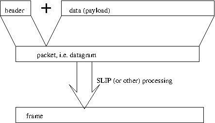
As an example of a very simplified IP protocol, when we have data to send on our network, we could place the IP destination address in the first 4 bytes of a packet, immediately followed by all the bytes of the data. The IP destination address should be placed with the "first" byte first, that is, 129.237.1.2 should be encoded so that 0x80 is the first byte, 0xAB the second, 0x01 the third, and 0x02 the fourth. The receiver of such a packet, assuming there were no errors, would then look up the first four bytes in its routing table, and forward the packet on towards its destination. The final destination would recognize its own IP address and understand that the packet is for itself. Perhaps a further protocol might then tell the recipient what to do with the data just received.
This very simplified protocol has two things in common with the true IP version 4 (IPv4) protocol: there is a separate header placed before the packet data, and the header includes the destination IP address. The header and the packet are sent as a single frame, as in the following figure.
The payload itself may consist of the header for a different protocol, followed by the data for that protocol. For example, frequently the payload of an IP packet is a TCP header followed by a TCP payload. The END character used in SLIP can be considered a trailer, though in SLIP a separate END character can also be sent as a header.
An IP packet is usually referred to as a datagram. Datagram is a generic term for packets used in connectionless communications, where each packet is sent independently of other packets.
One alternative to datagrams is the idea that successive packets might be related to each other in a meaningful way, usually sequentially. These packets give a stream of bytes, packets, or data.
The opposite of a connectionless communication is connection-oriented communication, which we will see when we discuss TCP. TCP is connection-oriented and provides the abstraction of sending and receiving a stream of bytes. IP and UDP are connectionless and support the exchange of datagrams.
In IPv4, the header is 20 bytes long (or more). The header includes both the destination address, which is used for routing, and the source address, which the recipient can use to reply to the message. These two addresses account for the last 8 of the minimum 20 bytes.
The original document defining IPv4 is RFC 791 (1981), at http://www.ietf.org/rfc/rfc791.txt. This RFC, and other RFCs defining TCP and other protocols, were updated by RFC 1122 (1989), at http://www.ietf.org/rfc/rfc1122.txt.
The IPv4 header actually begins with a 4-bit field recording the IP version number -- this is the value "4" for IP version 4. The next 4 bits are the IP header length, in units of 32-bits. For a 20-byte header, this value is therefore 5, and for a 20-byte header, the first byte takes the value 0x45 (decimal 69). If the header is longer than 20 bytes, it must be extended in a way that keeps the length a multiple of 4 bytes. For example, a header length of 24 bytes would be encoded by a first byte of 0x46, a header length of 28 bytes would be encoded by a first byte of 0x47, and the maximum header length of 60 bytes would be encoded by a first byte of 0x4F. The header length might be longer than 20 bytes if the sender has placed options at the end of the header. A number of options have been defined, but IP options are not used by most of the Internet traffic, for the following reasons. Having a variable-sized header with variable contents makes it harder for routers that forward packets efficiently, e.g. with assistance from specialized hardware. Also, some of the options are ineffective in today's Internet or have security implications that are not welcome in today's Internet.
The options may require an odd number of bytes. If the total size of all the options is not a multiple of four bytes, the header is extended to a 4-byte boundary. Keeping the header a multiple of four bytes has a benefit beyond reducing the number of bits used to store the header length. Most computers have a preferred alignment for data. In the most general case, bytes can have any alignment, 2-byte units (for example, values of type short int in C) should be aligned on a 2-byte boundary, 4-byte units should be aligned on a 4-byte boundary, and so on. The penalty for mis-alignment may be a loss of performance (typical on CISC architectures such as the x86) or bus errors (typical on RISC architectures such as SPARC or MIPS). IP and other Internet protocols are designed so that, if the IP packet header is stored in a buffer aligned on a 4-byte boundary, then the IP payload is also aligned on a 4-byte boundary. This restriction on where in memory fields should appear is known as an alignment restriction. Most of the Internet protocols require such alignment and in turn provide it to their payloads. One notable exception is Ethernet, which has a 14-byte header. One reason for this exception may be that Ethernet was designed to be implemented in hardware, whereas alignment restrictions make sense for implementations in software on general-purpose computers.
The second byte of the header is called type of service, and is another example (similar to IP header options) of a standard which is not widely used and perhaps not widely supported. The basic idea of type of service is to label packets as belonging to one of several classes:
Related to ToS is the Quality of Service (QoS), the performance of any network or system, generally as experienced by the endpoints of the network. For example, a video call might have a requirement for a specific bandwidth for each of the video and audio channels, and a requirement for a maximum delay of 100ms on the audio stream and 500ms on the video stream. Guaranteeing such QoS would require some sort of reservation of network resources, e.g. for each router that carries these audio and video streams, a reserved fraction of time spent forwarding packets on the appropriate interface.
Because the ToS field is not widely used, the low-order two bits have been re-purposed to indicate whether the sender wishes for any congestion to be recorded, and if so, whether the packet has experienced congestion. However, it is not clear that this extension is used any more commonly than the ToS field.
The 3rd and fourth bytes of the header are the total length of the IP packet. This is the length (in bytes) of the entire packet, including the header and the payload which follows the header. In our system, such a header could help us detect packets where one byte has been lost (we know this is a possible problem on serial lines). The length is stored as a 16-bit number, with the more significant byte stored first and the less significant byte stored second.
This storage strategy for the total length -- more significant bytes sent before less significant bytes -- is used throughout the Internet protocols and is referred to as big-endian binary encoding (the order of bits within a byte is generally standardized by the underlying hardware, and so does not affect networking software). The opposite strategy is called little-endian. People in the field sometimes strongly feel that one or the other approach is better, perhaps because they are accustomed to a machine architecture that favors one or the other -- for example, the Intel architecture is little-endian, but many other architectures are big-endian.
This kind of strong belief is similar to the religious wars satirized in Swift's "Gulliver's Travels", in which the inhabitants of one island, who open eggs at the big end, fight terrible wars with the inhabitants of a neighboring island, who open eggs at the little end. These two groups fight over which is the "right" end of the egg to open. There is, of course, no right or wrong side to an egg, as there is no right or wrong way of ordering the bytes of a 32-bit word.
To convert to and from big-endian order, also called network byte order, the function htons will convert a Short (a 16-bit integer) from Host format TO Network format, that is, to big endian format. htonl does the same for 32-bit integers. ntohs and ntohl perform the opposite conversion from network format to host format. These functions may be implemented as C macros. On machines whose native format is big-endian, these operations do nothing, but portable code which must run on both kinds of machines uses these functions to place values in the correct byte order.
As an example of the usage of this function, when we combine an Internet address and port number to give to the bind function we do:
int socket_fd = ...
unsigned short port_number = ...
struct sockaddr_in sin;

sin.sin_family = AF_INET;
sin.sin_port = htons(port_number);
sin.sin_addr.s_addr = INADDR_ANY;
if (bind (socket_fd, (sockaddr *) &sin, sizeof (sin)) != 0) { ... /* error */
We use the same structures to provide an address for a connect
call:
int socket_fd = ...
unsigned short port_number = ...
unsigned int ip_number = ...
struct sockaddr_in sin;

sin.sin_family = AF_INET;
sin.sin_port = htons(port_number);
sin.sin_addr.s_addr = htonl (ip_number);
if (connect (socket_fd, (sockaddr *) &sin, sizeof (sin)) != 0) { ... /* error */
In our code, we must always carefully keep track of whether a quantity is
in network byte order, which is what we send or receive on the network,
or in host byte order, which is what we can compare, increment, or
otherwise operate on. Most networking protocol use big-endian byte
order, though some protocols, such as Kerberos, allow either endianness.
In Kerberos, a bit in the header specifies which endianness is being used.
Endianness only applies to multi-byte quantities, and so doesn't apply to
ASCII based protocols such as HTTP (version 1), in which the information
is encoded as sequences of individual bytes.
The second 32-bit word of the IP header has to do with fragmentation, and will be discussed in Section 5. This section looks at the third 32-bit word of the IP header.
The 9th byte of the IP header is called Time-To-Live, and usually referred to as TTL. The original intent of this field was that it be decremented once a second. If the value should ever reach zero, the packet should be discarded. This keeps a single packet from "living forever", and forever consuming resources such as memory and bandwidth on transmission lines.
The clocks of different routers, however, are not necessarily synchronized. In addition, a router generally forwards a packet in a small fraction of a second. It was decided, therefore, that the TTL would be decremented once for every entire second that a packet spends on a host or router, and also once for every time that a packet is forwarded by a router, that is, traverses a "hop". The TTL field, therefore, is a combination of maximum hop count and actual time to live.
The TTL field is usually set to a standard value, for example 60 or 64, by the sender. Special applications can set particular values for the TTL. For example, an application called traceroute, described below, uses the TTL to automatically find out the route traversed by packets in the Internet. For another example, applications that want to make sure packets do not leave the local network (maybe for security purposes), can set a TTL of 1 so that no router will ever forward such packets.
The 10th byte of the IPv4 header is the protocol field. This field is used to answer the question, hinted at above, of what to do with the payload. The number in this field identifies a protocol that knows how to interpret the payload. A value of 1 identifies the Internet Control Message Protocol, ICMP, discussed below. A value of 6 identifies the Transmission Control Protocol, TCP, and a value of 17 (0x11) identifies the User Datagram Protocol, UDP, both of which are described in the next chapter. Many other values have been assigned, as documented starting on page 8 of RFC 1700, at http://www.ietf.org/rfc/rfc1700.txt. RFC 1700 is obsolete as of January 2002 (according to RFC 3232), and the current reference for assigned numbers is at http://www.iana.org.
The next two bytes of the header are a checksum for the header itself. The basic idea of a checksum is to add all the bytes in the header, and record the sum in the header itself. The receiver can then perform the same computation and verify that the header was received without errors. Checksums are easy to compute (just add the numbers together), but do not provide as much protection against errors as stronger algorithms such as Cyclic Redundancy Checks (CRCs), which are discussed in Chapter 3. For example, if two numbers in a sum are exchanged (A+B vs. B+A), the total will remain the same even though the header has changed and may now be meaningless.
The Internet checksum adds all pairs of bytes using 1's complement arithmetic. When checksumming an odd number of bytes, a 0 byte is added at the end for the calculation, but this is never a concern with the IP header.
In 1's complement arithmetic, the complement (negation) of a number is obtained by inverting each bit of the number.
One reason why one's complement arithmetic is not more widely used in computers is, there are two representations for the number 0, 00000... and 11111...
Some of the mathematical properties of the Internet checksum are discussed in RFC 1071, at http://www.ietf.org/rfc/rfc1071.txt. For this discussion, suffice it to say that most modern computers do not provide 1's complement arithmetic, but can implement it relatively easily. The 16 bit, 1's complement sum of a set of numbers is the (normal) 16-bit sum of those numbers, added to any carry from the 16-bit sum. For example, the sum of the 16-bit numbers 0x89AB + 0xCDEF = 0x1579A, a 17-bit number. Adding the carry back in gives us 0x579B, which in this case is the checksum result given by step 4 below. In step 5 we invert this, giving 0xA864.
A sender of an IP packet takes the following steps:
The receiver performs steps 3 and 4 and, if the result is 0xFFFF, knows the header has no detected errors.
The reader is encouraged to practice verifying the IP checksums of the headers in examples 1 and 2, to detect which of the two has bit errors (one is correct, and the other one has errors). Another useful practice is to compute the correct Internet checksum for the third packet header shown. In all these examples, the packet payloads are not shown, as they do not affect the computation of the checksum. All numbers are given in hexadecimal. The bytes of a word are read from left to right, and successive words follow from top to bottom.
45 00 01 23 45 67 00 00 03 06 8D 15 12 34 56 78 9A BC DE F0 |
45 00 02 34 56 78 00 40 29 11 56 A8 12 34 56 78 9A BC DE F0 |
45 00 02 34 56 78 00 00 29 11 56 E8 12 34 56 78 9A BC DE F0 |
In addition to the fields described above, the IP header includes a source IP address and a destination IP address, so the overall structure of the IP header is (from RFC 791):
 0                   1                   2                   3
 0 1 2 3 4 5 6 7 8 9 0 1 2 3 4 5 6 7 8 9 0 1 2 3 4 5 6 7 8 9 0 1
+-+-+-+-+-+-+-+-+-+-+-+-+-+-+-+-+-+-+-+-+-+-+-+-+-+-+-+-+-+-+-+-+
|Version|  IHL  |Type of Service|          Total Length         |
+-+-+-+-+-+-+-+-+-+-+-+-+-+-+-+-+-+-+-+-+-+-+-+-+-+-+-+-+-+-+-+-+
|         Identification        |Flags|      Fragment Offset    |
+-+-+-+-+-+-+-+-+-+-+-+-+-+-+-+-+-+-+-+-+-+-+-+-+-+-+-+-+-+-+-+-+
|  Time to Live |    Protocol   |         Header Checksum       |
+-+-+-+-+-+-+-+-+-+-+-+-+-+-+-+-+-+-+-+-+-+-+-+-+-+-+-+-+-+-+-+-+
|                       Source Address                          |
+-+-+-+-+-+-+-+-+-+-+-+-+-+-+-+-+-+-+-+-+-+-+-+-+-+-+-+-+-+-+-+-+
|                    Destination Address                        |
+-+-+-+-+-+-+-+-+-+-+-+-+-+-+-+-+-+-+-+-+-+-+-+-+-+-+-+-+-+-+-+-+
|                    Options                    |    Padding    |
+-+-+-+-+-+-+-+-+-+-+-+-+-+-+-+-+-+-+-+-+-+-+-+-+-+-+-+-+-+-+-+-+
The destination IP address is what we started with: it is the main feature of the header that allows the packet to be delivered to the intended host. The source IP address is less immediately useful, though it does allow applications to respond to incoming messages.
Any host in the Internet can send a packet to any destination on the Internet. If the destination address is not a valid address for a host, eventually it will reach a router that does not have a routing table entry for that destination, and that router will discard the packet.
The source address field is normally set to a valid source address for the sending host. In theory, a host could send IP packets with invalid, or spoofed source IP addresses. This is sometimes done by packets in denial of service attacks, though it can also be useful for legitimate purposes. Routers at the boundary of a network may check to make sure that packets forwarded from inside the network carry a source IP address that is valid inside the network, and discard packets with spoofed source addresses -- this is called egress filtering.
A C structure that captures the layout of the IPv4 header might look as follows. To understand the fragmentation fields, refer to section 5.
struct ipv4_header {
  uint8_t ver_hlen;    /* version and header length, usually 0x45 */
  uint8_t tos;         /* type of service */
  uint16_t length;     /* total packet length */
  uint16_t packetid;   /* packet ID */
  /* flags_frag has 3 flag bits, then 13 bits of fragment offset */
  /* the 3 flag bits are, in order, reserved (always zero), Don't Fragment,
     and More Fragments, as seen in the next two constants */
#define IP_DONT_FRAGMENT_BIT    0x4000
#define IP_MORE_FRAGMENTS_BIT   0x2000
  /* the fragment offset is 1/8 of the offset of this fragment, in bytes */
#define IP_FRAGMENT_OFFSET_MASK 0x1FFF
#define encode_fragment_offset(offset_in_bytes) ((offset_in_bytes) >> 3)
#define decode_fragment_offset(offset_from_packet) \
                 (((offset_from_packet) & IP_FRAGMENT_OFFSET_MASK) << 3)
  uint16_t flags_frag; /* 3 flag bits, then 13 bits of fragment offset */
  uint8_t ttl;         /* time to live */
  uint8_t protocol;
  uint16_t checksum;
  uint32_t source;
  uint32_t destination;
  /* the following array with zero characters can be used because C doesn't
     check for array bounds violations, so we can actually access locations
     with index higher than -1.  The programmer MUST however ensure
     that enough memory has been allocated.  IP also requires that the
     number of option bytes be a multiple of four. */
  uint8_t options [0];
}
Finally, there are two basic steps that a host performs when a packet is first originated:
The major concern was the growth of the IPv4 network. IPv4 addresses are only 32 bits long, and that limits the maximum size of the Internet, as will be seen in Sections 8 and 9 of this chapter. Instead, IPv6 addresses are each 128 bits (16 bytes) long. Each IPv6 header has a source and a destination IP address, for a total of 32 bytes, preceded by 8 other bytes, giving a 40 byte fixed-size header.
Header fields of IPv6 that resemble fields of IPv4 include:
The last two are further discussed below, together with a totally new 20-bit field called a flow label.
Notably missing is any support for fragmentation and header checksums. Fragmentation will be discussed below. Header checksums were thought to be of limited use, and omitted to simplify the implementation of routing functions directly in hardware.
The header format is described in RFC 2460, which is the basic specification for IP v6.
+++++++++++++++++++++++++++++++++
|Ver| Class |      Flow Label   |
+++++++++++++++++++++++++++++++++
|Payload Length |Nxt Hdr|Hop Lmt|
+++++++++++++++++++++++++++++++++
|                               |
+                               +
|                               |
+         Source Address        +
|                               |
+                               +
|                               |
+++++++++++++++++++++++++++++++++
|                               |
+                               +
|                               |
+       Destination Address     +
|                               |
+                               +
|                               |
+++++++++++++++++++++++++++++++++
struct ipv6_header {
  uint8_t ver_class_hi; /* version and 4 bits of class, usually 0x60 */
  uint8_t class_lo_flow_hi; /* 4 bits each of class and flow label */
  uint16_t flow_lo;     /* 16 bits of flow label */
  uint16_t length;      /* payload length */
  uint8_t next_header;  /* next header: TCP, UDP, ICMP, or extension */
  uint8_t hop_limit;    /* same as IPv4 TTL */
  uint8_t source [16];  /* source address */
  uint8_t destination [16];  /* destination address */
}
The version number is always six and takes up the first 4 bits in the datagram, as in IPv4. The next 8 bits are the traffic class -- this is the only header field that is not aligned, spanning two different bytes. The traffic class is not defined by the RFC, except to say that zero should be the default. The intent is that the traffic class is analogous to the IPv4 Type of Service field -- even though ToS is not widely used, the designers of IPv6 decided to retain it.
The flow label takes up the next 20 bits. The idea of a flow label is to allow routers and hosts to negotiate special properties for a sequence of related packets -- for example, special routing or special low-latency delivery. The combination of flow label, source address, and destination address identifies packets belonging to a given flow. We further discuss flow labels in section 7.4.6.
Payload length is the length, in bytes, of the datagram, minus the forty bytes of the IPv6 header. The maximum length is 216 bytes, though there are also mechanisms for supporting longer datagrams.
Next-header identifies the first header in the payload. This could be a transport-level protocol, such as ICMP, TCP, or UDP, or an IP extension header. The IPv6 header size is constant, so there is no room in the IPv6 header for options. Instead, IPv6 has defined a number of extension headers. Extension headers include hop-by-hop headers, which must be processed by every router, and end-to-end headers for fragmentation, security, and authentication. The headers must appear in a specified order: first the hop-by-hop headers (processed by every router), then fragmentation, security, and authentication headers (only processed by the destination), and finally any other "destination" headers (end-to-end headers). The hop-by-hop and destination options are specified in an extensible manner, with a length and a code field that specify what routers or hosts should do if they do not recognize the extension header, specifically one of:
This allows the introduction of new options with a predictable effect.
The following figure shows an IPv6 header, followed by an extension header -- in this case, a routing extension header -- followed by the IPv6 payload -- in this case, a TCP segment, consisting of a TCP header and TCP payload.

Because each IP address is made up of a network part and a host part, the IP address depends on the network to which an IP host or router is connected. For example, if I connect a host to the network 1.2.3.0, and if the network part is the leftmost 24 bits of the address (i.e. the 3 bytes 1.2.3 are the network part of the address), then the only IP numbers I may be able to use are 1.2.3.0, 1.2.3.1, 1.2.3.2, and so on up to 1.2.3.255. Any other IP address does not belong on this network.
The fact that the IP number is based on the network number has two consequences. The first is that the IP number cannot be assigned to a computer by the manufacturer, but must be configured at the time the computer is connected to the network. The second consequence is that a multihomed host, and therefore a router, must have different IP addresses on each of its interfaces. An example of this is shown in the following figure, where the notation a.b.c.d/B means the address is a.b.c.d, and the network part of the address is B bits.
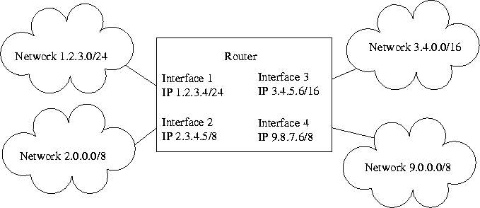
It should be clear that there is no single "router IP address", only addresses for each of the router's interfaces. To be consistent, a multihomed host replying to a message received on a given interface usually tries to use as a source address the IP address of that interface, but this is not always the case.
There are two special IP addresses on every network. Both of these addresses have the same network part. If the host part is all zeros, this is the network address. It is not really meant as a potential destination address, rather it is used to refer to the network itself, and can appear, for example, in a routing table.
If the host part of the address has every bit set to 1, this is the network broadcast address, or simply the broadcast address. This can be a destination address, implying that every host on the network is the destination of a given packet, but should never be used as a source address. Neither the network address nor the broadcast address should be used as a host address. As a result, a network with a 24-bit network part and an 8-bit host part can have at most 254 different hosts on it, numbered 1..254.
The original definition of IP version 4 had a very simple algorithm for determining the number of bits in the network part of the address:
As might be suspected, there are also class D addresses (initial bits 1110), used for multicasting, and class E addresses (initial bits 1111), which are reserved.
This class-oriented addressing scheme is very effective in the sense that routers can easily compare the network number in the destination address of a packet to network numbers stored in its routing table. At the extreme, a router might (internally) keep three routing tables, one for class A, one for class B, and one for class C addresses, and use very fast searching techniques to locate a given address in the routing table.
The drawback of class-oriented addressing is that it is inflexible. There is only a two-level hierarchy, since it is not possible to have networks and subnetworks. Also, if one wishes to obtain an IP address for a network with 254 or more devices, or a network that might potentially grow to have more than 254 devices, one needs a class B address, and there are only 16,384 possible class B addresses. These two issues led to the development of two different solutions. The first solution is IP version 6, and addressing for IP version 6 addresses is discussed in section 4.3. The second solution was meant as an interim solution, and is the development of network masks and classless inter-domain routing (CIDR), described in Section 4.4.
Finally, some of the addresses in each class are reserved (by RFC 1918) for private use, that is, should never be routed on the public Internet. These include the class A network 10.0.0.0 (10/8), the class B networks 172.16.0.0 through 172.31.0.0 (172.16/12), and the class C networks 192.168.0.0 through 192.168.255.0 (192.168/16).
In the first place, IPv6 addresses are much longer than IPv4 addresses, and are written differently. They are written using hexadecimal instead of decimal, using groupings of 16 bits rather than groupings of 8 bits, and using colons to separate the groupings rather than dots. Further, any single sequence of zero groupings can be replaced by a double colon, so that all the following are IPv6 addresses (from RFC 2373):
1080:0:0:0:8:800:200C:417A or 1080::8:800:200C:417AAddress prefixes can also be represented, as in the following legal representations of the 60-bit prefix 12AB00000000CD3 (again, from RFC 2373):
FF01:0:0:0:0:0:0:101 or FF01::101
0:0:0:0:0:0:0:1 or ::1
0:0:0:0:0:0:0:0 or ::
12AB:0000:0000:CD30:0000:0000:0000:0000/60
12AB::CD30:0:0:0:0/60
12AB:0:0:CD30::/60
The specific rules are in the RFC.
Most of the IPv6 address space is currently unassigned. As in the classical IPv4, classes of addresses in IPv6 are identified by specific values of the first few bits (at most 10) of the address. Those classes that have been defined include:
In addition to this motivation, organizations that already had class B addresses assigned found that they were running multiple networks, and wanted to connect these internal networks with routers. In other words, these organizations found they needed to have a two-level hierarchy within their own networks, leading to an Internet where the addresses were part of a multi-level hierarchy. In other words, the Internet was becoming not just a two-level hierarchy, but a three- or four-level hierarchy. This meant giving up class-based addressing in favor of a different mechanism, one which is now referred to as Classless Inter-Domain Routing, or CIDR (pronounced like the word "cider").
In order to accomodate this change, the concept of a network mask was standardized. A network mask identifies the network part of an IPv4 address. For example, in the class-less world the IP address 1.2.3.4 might be given a 22-bit network part, and consequently a 10-bit host part. The network part would be written 1.2.0.0/22. The corresponding network mask has 22 bits of ones on the left, and 10 bits of zeros on the right, and is therefore written, in dotted-decimal notation, as 255.255.252.0.
To obtain the network part of an address, i.e. the network number, the computation is now as follows. Given an address A and a mask M, the network number is the bitwise AND of A and M.
It was noted in Section 2.7 that in order to determine whether a packet can be delivered directly to the destination, a host or router must determine whether it is directly connected to the destination network. In order to do so, the host or router must have an address mask associated with each of its IP numbers, that is, an address mask associated with each of its interfaces. There is no requirement that these address masks be the same -- if a host's two interfaces are (1) on a point to point link, and (2) on a large Ethernet, the corresponding address masks might be 255.255.255.252 (30 bits) and 255.255.0.0 (16 bits).
Section 2.7 also mentioned, and Section 7 will explain in detail, that in order to route a packet, the network number of the destination address must be matched against the network numbers of all the routes in the routing tables. However, a router generally does not know the appropriate network mask for a given destination. Instead, a router using CIDR keeps a network mask for each route. The destination address is then masked with each route's network address, as follows. Given a packet destination address D, a route address A and mask M, the route matches the packet if the bitwise AND of D and M is equal to the bitwise AND of A and M.
With this system, it is very easy to represent the default route as simply a route with an arbitrary destination A, and a network mask of 0.0.0.0. As a result, different routes may match a single destination address D. The proper way to select a route in this case is to select the matching route that has the longest network mask, that is, the network mask with the largest number of one bits. This selection is easy to perform on conventional computers by simply selecting the matching route with the numerically largest network mask.
A sample routing table might be:
% route -n
Kernel IP routing table
Destination     Gateway         Genmask         Flags Metric Ref    Use Iface
0.0.0.0         129.237.15.1    0.0.0.0         UG    100    0        0 eth0
129.237.15.0    0.0.0.0         255.255.255.0   U     100    0        0 eth0
169.254.0.0     0.0.0.0         255.255.0.0     U     1000   0        0 eth0
In this case, the first entry of the routing table shows the default route, and the gateway for the default route is 129.237.15.1.
Similarly, a sample IPv6 routing table might be:
% route -6n
Kernel IPv6 routing table
Destination                    Next Hop                   Flag Met Ref Use If
::1/128                        ::                         U    256 1     0 lo
2349:abcd:4444:77::/64         ::                         U    100 3548908 eth0
fe80::/64                      ::                         U    100 3128682 eth0
fe80::/64                      ::                         U    256 1     0 eth0
::/0                           2349:abcd:4444:77::1       UG   100 3187281 eth0
::1/128                        ::                         Un   0   4   825 lo
2349:abcd:4444:77:123:4567:89ab:cdef/128 ::                         Un   0   41750304 eth0
fe80::9876:5432:10fe:dcba/128  ::                         Un   0   4315416 eth0
ff00::/8                       ::                         U    256 3625907 eth0
::/0                           ::                         !n   -1  1     1 lo
In this case, the default route is the fifth routing table entry, with a next-hop address (i.e. gateway) of 2349:abcd:4444:77::1. You can see that the network number of this next hop matches the network number shown in the destination field of the second route.
The very first route in this table (and for some reason, also the fifth) is the loopback address, and the very last route is a dummy entry that discards any packets that don't match any other routes.
Having discussed network masks we now look at how they are used. Consider an organization that has been assigned a class B address, for example a university. Any router outside of this university can still route using class-based addressing, and deliver packets to one of the routers at this university. If the routers outside the university are using CIDR, they will be using an address mask of 255.255.0.0, which is the network mask for a class B address.
Within this university, the network administrators have decided to assign to each sub-network a 9-bit sub-network number, leaving 7 bits for each host number. That is, each host and router will be configured with a network mask of 255.255.255.128 for any address within this university's class B. A host on one of these networks will then know that if the first 25 bits of an address match the host's own IP address, the communication can proceed directly over the local network, and otherwise packets will have to be sent to the local default router.
CIDR offers much more flexibility than the above example illustrates. Network administrators could choose to assign different numbers of bits to different subnetworks, allowing some to grow larger than others. An ISP might obtain a sequential set of class C addresses, and combine them all into what a supernet -- that is, a single IP network that was originally assigned as several networks. A user with a small home network can obtain 8 or 16 "host" IP numbers from an ISP and form them into a supernet, requiring a router between the home network and the ISP.
CIDR is a way to use addresses, especially IPv4 addresses, more efficiently. There are other ways of increasing the efficiency of our address usage. One strategy that is common for home networks connected through an Internet Service Provider (ISP) is to connect several different computers to the Internet using a single IP address. To do this, we must provide a Network Address Translation system, or NAT box, which connects to an internal network on one interface, and to the Internet on a different interface. Both interfaces use IP to communicate. Addresses of interfaces on the internal network are non-routable IPv4 addresses such as 10.*.*.* or 192.168.*.*, whereas the address of the external interface is the IP address assigned by the ISP.
Communications within the internal network proceed as usual. However, whenever an internal computer tries to send a message outside the internal network, the NAT box must rewrite the IP header so the source address is its own external IP number. The NAT box is also responsible for remembering that it has done this, so that when a reply comes, the destination address can be changed to match the internal IP address of the system that first sent the packet. In this way, the internal host can connect to external hosts and communicate almost as if it was on the Internet. The only limitation is that hosts on the Internet cannot initiate connections to hosts within the home network unless the NAT box has been manually set up to allow this to happen. For many users, this limitation is actually a security feature, preventing a variety of network attacks.
To do all this reliably, the NAT box must use information not present in the IP header. For example, internal systems A and B might both send a packet to the same outside web server -- the responses should be delivered correctly to either A or B, but not both. However, the IP header offers no information that would help distinguish between packets that are responses to A and packets that are responses to B. So the NAT system must use and rewrite not only the source and destination addresses, but also information provided by higher-level protocol which is sufficient to distinguish such packets. In the case of the TCP and UDP higher-level protocols, such information is called source and destination port numbers.
Network Address Translation is often combined with the firewall function, which consists of examining incoming packets (and sometimes outgoing packets) to try and prevent network attacks. Port numbers are used in such cases also, since connections from outside to some sets of port numbers are less likely to be legitimate and more likely to be network attacks.
Both IPv4 and IPv6 have mechanisms to allow a single large datagram to be divided into smaller datagrams if the MTU on a network does not allow the original large datagram to be sent in one frame. In IPv4, both hosts and routers can fragment a datagram, in IPv6 only the sending host fragments datagrams.
Fragmentation means that IP packets up to the maximum size can be sent even if the underlying network does not support this. Let us use as an example our SLIP network with an MTU of 1006 bytes, and an application wanting to send a UDP packet that is 4096 bytes long. Adding the standard 20-byte IPv4 header gives a total of 4116 bytes. Each fragment will need its own IP header, so the maximum number of payload bytes that a single fragment can carry is 1006 - 20 = 986. Since 4096 / 986 is 4.15, a minimum of at least 5 fragments will be needed to carry the entire payload.
If we want to send IP packets with IP header options, the computation is more complicated, since some options are carried with every fragment, and other options are only sent with the first fragment. If there is no requirement to send maximum-sized packets, one could assume that the IP header is 60 bytes or fewer, and simply use MTU-60 as the maximum fragment size.
How many bytes each of the 5 fragments carries is up to the implementation, as long as the following rules are observed. In what follows, L is the total length of the IP packet, 4116 in our example, h is the header length, 20 in our example, and M is the MTU of the network, 1006 in our example. Subscript i identifies fragments of the original datagram, and n the number of fragments, 5 in our example.
With an IP header length of 20 bytes, the total datagram length will not be a multiple of 8 (since 20 bytes is not a multiple of 8). It is the payload length that matters. Again, the final fragment may have an odd length. This last fragment has the MF (More Fragments) flag set to 0, whereas every other fragment carries MF=1. This flag is called M in the IPv6 Fragment extension header.
Any datagram or fragment may have the Don't Fragment (DF) bit set. If the bit is set (DF = 1), the datagram/fragment should not be further fragmented, and if fragmentation is required, the packet should be discarded instead. The IPv6 extension header that supports fragmentation does not have this bit -- instead, all IPv6 datagrams can only be fragmented by the original sender, and not by routers. The IPv6 routers therefore can only discard a received packet that does not fit in the MTU.
Fragments belonging to the same original datagram should all have the same ID field, the same source and destination address, and the same protocol field. Fragments belonging to different original datagrams should differ in at least one of these fields, most commonly the packet ID.
Although bytes on a serial line are transmitted in order, there is no guarantee that packets on an IP network will be received in the same order as they are transmitted. In particular, a router may arbitrarily reorder the packets it receives before resending them, perhaps because it believes some of them to be higher priority than others. A router may also send successive packets along different routes, so that a packet transmitted later may actually be received earlier.
In addition, there is no guarantee that all the packets sent will be received. Routers can discard packets for any number of reasons. Most frequently, a router will discard packets if it is receiving more packets than it can forward in a reasonable time.
IP reassembly is complicated by having to deal with packets that may not arrive in order, or may not arrive at all. Two strategies to deal with these issues are:
The first strategy insures that a missing fragment does not cause the other fragments to consume resources forever. The second strategy insures that arbitrary reorderings will not interfere with successful reassembly.
In implementing the first strategy, how do we know when we have received a fragment for a new packet? We know we are looking at a fragment, rather than a complete packet, if the fragment offset is nonzero, or if the MF flag is 1. Conversely, if both the fragment offset and MF are zero, we know this is the first fragment (FO = 0) and also the last and therefore only fragment (MF = 0), so this must be a complete packet.
If we know we have a fragment, how do we know if it is a fragment for an existing packet that we are reassembling, or a new fragment for a new packet? The answer is that every datagram sent by an IP host to a given destination address should bear a different packet ID number. Since there are only 16 bits in the packet ID field, these numbers will have to be recycled after sending at most 216 packets, but this distance should be sufficient to minimize the chance of integrating fragments from different packets into the same reassembled packet. The easiest way to generate different packet IDs is to increment a 16-bit number, though the RFCs do not specify a given mechanism, and indeed other algorithms are possible.
Finally, what algorithms and data structures should we use to reassemble packets no matter what order the fragments are received in? The answer to this is beyond the scope of these notes. A particularly well thought-out answer is presented by RFC 815, http://www.ietf.org/rfc/rfc815.txt . In brief, the Clark algorithm described in RFC 815 keeps track not of the fragments received, but of the parts of the packet that are yet to be filled. A particularly clever part of the algorithm uses memory space of the storage buffer that the reassembled packet will be stored in to store the data structure itself. This minimizes copying, dynamic allocation, and the likelihood of memory overflow or memory leaks, all important considerations in a real system.
The basic algorithm for reassembly is as follows:
Basic IP processing is relatively easy to program correctly. However, in any protocol the features used least frequently tend to be the least tested, and this is true for IP as well. An example of this is the fragmentation mechanism. The maximum size of an IPv4 packet is defined to be 216 bytes, so a network implementer could allocate a buffer of 216 bytes to hold packets for reassembly. However, the fragment offset of an IP fragment can be as much as 216-8, or 1111 1111 1111 1000 (0xFFF8), remembering that the least significant three bits are always zero and are not sent. Unfortunately, this means someone could send a fragment with an offset of 0xFFF8 and a size greater than 8. If a network implementer were to copy such a fragment into the buffer without checking, the buffer would overflow and the contents of the fragment could corrupt operating system data structures.
Such a fragment could never be created in the process of fragmenting a legal IP packet, however large. Such a fragment would be created in the course of a deliberate attack on a network-connected system. There is a class of IP packets accepted by many systems called a ping packet, and this attack has come to be known as the ping of death, since the affected machines often would lock up.
Other strange things can happen during reassembly. If a packet is duplicated by the network, it may be that a received fragment overlaps part of the packet that has already been received. Either the old or the new fragment could be used, though customarily the old one is retained. It is always interesting to speculate on the appropriate action to take if the contents of the new and old fragments (at the same fragment offset) should differ. Duplication can also cause fragments to overlap already-received fragments -- consider a packet being duplicated, with the two copies sent along different routes, with the copy sent along one of the routes being further fragmented, and some but not all of those sub-fragments being lost.
In general, IP does not guarantee that the contents of a packet have been delivered correctly. This task is usually left to higher-level protocols such as TCP and UDP. TCP for example will retransmit any packet that has been corrupted during delivery. It is therefore appropriate for IP to simply do a best-effort job of delivering the packet, and not worry about whether, for example, different overlapping fragments all have the same contents.
The simplest answer is that all links in the Internet are required to carry packets of size at least 1280 bytes. This is true for IPv6, whereas the original IPv4 only required an MTU of 576 bytes. This would mean that for our SLIP network to carry IPv6 packets, we would have to increase the MTU from 1006 bytes to at least 1280 bytes. For the implementation shown in Chapter 1, all this requires is modifying a constant and recompiling.
Alternatively, an IPv6 sender may simply try to send bigger packets. If a router discards the packet because it is too large to send on a given link, the router is supposed to create a message and send it back to the sender explaining why the packet was dropped. The sender can then reduce the maximum size of packets sent, perhaps by using IPv6 fragmentation. This process is called Path MTU discovery, and is described by RFC 1981 for IPv6, or RFC 1191 for IPv4.
The packet that the router sends back to the sender, notifying the sender that the packet was dropped, is defined by a protocol called ICMP, discussed in the next section.
On a point-to-point link, debugging the network is relatively easy. Whether the packets are not going through, or whether packets are lost or corrupted, the fault can generally be traced to either hardware or the software on the two sides of the link.
Debugging an Internet is harder. If packets get lost, there may be no indication of where they are getting lost. The systems involved may be thousands of miles apart, and even if they were nearby, it is unlikely my ISP's backbone provider would agree to let me inspect their routers to verify that their routing software and hardware are working correctly. Instead, we need ways to use the network to debug the network. More specifically, we need to be able to use the parts of a network that work to debug the parts of a network that aren't working very well. The protocol used to do this is called the Internet Control Message Protocol, or ICMP. ICMP packets are IP packets with a protocol number of 1. The ICMP header and payload form the payload of the IP packet. ICMP is defined by RFC 792, at http://www.ietf.org/rfc/rfc792.txt.
The most basic way to debug the network is to send a packet to another host, and have the host respond. If the response is received, the network has successfully delivered at least this pair of packets. Repeating the procedure will give us an idea of the loss rate between these two hosts. In addition, we can put a timestamp into outgoing packets. If the destination host copies the timestamp into the packet that they send back, then the original sender can measure the round-trip time of the connection. The program which does this is called ping, and this kind of packets is often called a ping packet, though the official ICMP names for these packets are ECHO and ECHO REPLY. The format of ICMP echo and echo reply packets is defined in RFC 792:
 0                   1                   2                   3
 0 1 2 3 4 5 6 7 8 9 0 1 2 3 4 5 6 7 8 9 0 1 2 3 4 5 6 7 8 9 0 1
+-+-+-+-+-+-+-+-+-+-+-+-+-+-+-+-+-+-+-+-+-+-+-+-+-+-+-+-+-+-+-+-+
|     Type      |     Code      |          Checksum             |
+-+-+-+-+-+-+-+-+-+-+-+-+-+-+-+-+-+-+-+-+-+-+-+-+-+-+-+-+-+-+-+-+
|           Identifier          |        Sequence Number        |
+-+-+-+-+-+-+-+-+-+-+-+-+-+-+-+-+-+-+-+-+-+-+-+-+-+-+-+-+-+-+-+-+
|     Data ...
+-+-+-+-+-
The type field must be 8 for echo messages, 0 for echo reply messages. For ping packets, the code field always has the value zero. The checksum is computed in the same way as the IP header checksum, but covers the entire packet. The identifier is set to a number that uniquely identifies the sending program on the sender -- in Unix, this is the process ID of the ping. The sequence number is normally incremented as packets are sent. To see this in action, simply run the ping program on almost any machine, specifying the destination machine. Depending on your operating system, you may also have to specify certain switches that will allow you to see what the ping program is doing -- study your available documentation carefully to find out.
Logically, the recipient copies the identifier and sequence number from the echo to the echo reply message, and sends it back to the sender. In practice, there is no need to copy. The recipient can simply replace the type field and send the packet right back. We can imagine coding a data handler that would do this.
static void icmp_data_handler (unsigned long from_ip,
                               char * data, int data_length) {
  if ((data_length >= 8) && (check_icmp_checksum (data, data_length))) {
    if (*data == ICMP_ECHO_TYPE /* 8 */ ) {
      *data = ICMP_ECHO_REPLY_TYPE; /* 0 */
      compute_icmp_checksum (data, data_length);
      ip_send (from_ip, data, data_length);
    } else if (*data == ICMP_ECHO_REPLY_TYPE /* 0 */ ) {
      unsiged short id  = * ((unsigned short *) (data + 4));
      unsiged short seq = * ((unsigned short *) (data + 6));
      /* deliver the packet wherever it is supposed to go */
      icmp_echo_reply_handler (id, seq, data + 8, data_length - 8);
    } else ... /* many other possible ICMP types */

  } else {
    /* bad checksum, do nothing (i.e., discard the packet) */
  }
}
In the above code I have assumed the existence of appropriate checksum functions. These can at their core have the same checksum function that is used to checksum the IPv4 header, though on many systems the IPv4 header checksum computation is very highly optimized, in which case the code may be different.
In the above code I have also assumed the existence of a function called icmp_echo_reply_handler, which keeps a database of ID numbers and information about what to do with echo reply packets received for each such ID number. How this database is implemented can vary a lot, though the simplest way is to keep a table in memory analogous to the routing table. At any rate, this icmp_echo_reply_handler must be able to tell a ping program when an echo reply is received, what the sequence number was, and deliver the data to the ping program.
How the data is given to the user program is very specific to each operating system. You don't need to know how this works, but if you are curious, you can read the remainder of this paragraph. On Unix for example, the ping program would be blocked on a recv or recvfrom call on a special IP-level socket. More specifically, a single thread of the ping program would be blocked on such a call, since a ping program might be multithreaded. This means the operating system would have a structure with a pointer to the stack for this thread, and the thread would not be executable, that is, would never be considered by the operating system scheduler. The operating system includes the icmp_echo_reply_handler function. This function must copy the received data into the application's buffer, which is accessible from the thread's stack, then copy the return value for the call directly into the call stack. Finally, the operating system must mark the thread as executable, so that the scheduler can execute it. More details of this kind of operation should be available from any operating system implementation book or course. Many people refer to this operation as a context switch, assuming that the operating system restarts the thread immediately without waiting for the scheduler to schedule the thread.
Ping packets are the only class of ICMP packets that is normally sent directly by an application. Most other ICMP packets are sent by routers when an error or an unusual condition is detected. One example is the Path MTU discovery process mentioned above. When a packet is discarded, the router is supposed to send an ICMPv6 "Packet Too Big" message back to the sender of the original IP packet that is being discarded. The recipient of this packet thus knows that the given packet size is not supported, and can try to fragment future packets to fit within the available size.
Such ICMP error packets generally carry with them at least the IP header and the first 8 bytes of the IP payload of the packet that was discarded. Most protocols, including specifically TCP and UDP, can use this information to figure out exactly which packet was discarded, and take appropriate action.
One particularly useful (and common) kind of ICMP error packet is known as destination unreachable. When a router must discard a packet because it has no route to the destination, such a router will often send back an ICMP destination unreachable packet to inform the sender. The destination unreachable has different codes that specify whether the entire network was unreachable, or only the specific host. Additional codes can be used by a host receiving a packet with a protocol number that the host does not support, or for which there is no server on the specified port.
Another kind of ICMP error packet is the time exceeded message, which is used to report that a packet was discarded due to a TTL of zero.
Time exceeded messages are used by another user-level program called traceroute. This program takes as argument a destination IP address or DNS name, and starts to send UDP packets to this IP address. However, the first three packets sent are sent with a time-to-live value of one, and therefore will be discarded by the first router they find. Each of these discard should produce a time-exceeded message from the router back to the host, and traceroute faithfully prints out the IP address of this router. Then traceroute sends three more packets with a time-to-live of two, so the second router can now be expected to send time-exceeded messages, which traceroute can use to print the IP address of the second router. Continuing on, traceroute is eventually able to print the IP addresses of all the routers between this host and the destination that are willing to send time exceeded messages. Some routers, however, are configured not to send ICMP messages, and traceroute will not detect these. You can see this at 6 hops in the following traceroute, which uses IPv6 (IPv4 is similar -- try both!)
% traceroute -6n www.ietf.org
traceroute to www.ietf.org (2400:cb00:2048:1::6814:55), 30 hops max, 80 byte packets
2349:abcd:4444:77::/64
 1  2349:abcd:4444:77::1  1.061 ms  1.049 ms  1.040 ms
 2  2349:abcd:4444:3129::1  0.632 ms  0.800 ms  0.795 ms
 3  2349:abcd:0:1::1  1.426 ms  1.415 ms  1.403 ms
 4  2349:abcd:0:17::1  1.401 ms  1.549 ms  1.379 ms
 5  2349:3401:1::40:abcd:ef01  49.042 ms  49.030 ms  49.006 ms
 6  * * *
 7  2001:468:e00:801::2  49.503 ms  49.271 ms  49.451 ms
 8  2001:504:0:3:0:1:3335:1  50.295 ms  50.696 ms  50.257 ms
 9  2400:cb00:12:1024::ac44:2cf7  49.463 ms 2400:cb00:12:1024::a29e:386b  49.456 ms 2400:cb00:12:1024::ac44:d233  49.439 ms
Also note that the last hop has several different addresses, and each of them replies in turn.
ICMP has been carefully designed to avoid overloading the network under study. For example, hosts and routers are encouraged to limit the rate at which they will send ICMP error messages or respond to pings. In addition, no host or router is ever supposed to send an ICMP error message when dropping another ICMP error message -- this is similar to the TTL mechanism in preventing unlimited usage of resources for a single packet.
ICMP has been used in network attacks. One particularly effective denial of service attack consists in sending ICMP echo packets to a large number of internet nodes. Assume that the node under attack is node A, and the attacking node is node C. C sends ICMP echo packets to a large number of nodes B, but spoofing the source address so A appears instead of C. If C's router is willing to transmit these messages, the hosts B will all send ICMP echo reply packets to A, thereby slowing down A's network access. A has no effective way of detecting C, since A only received packets from the B nodes.
This attack would become impossible if every router, and in this example the router for A, would drop all packets that do not have a source node belonging to one of its networks, in this case C and other addresses with the same network number. Doing so constitutes egress filtering, which is useful but only prevent a subset of possible network attacks.
Although so far we have only been supporting point-to-point connections along serial lines, we want our routing tables to support more general configurations. In particular, we want to be able to use arbitrary "lower layer" networks to connect our computers. Some of these will be described in Chapters 4 and 5, but for now we simply need to be aware that these networks allow the interconnection of more than two computers, and hence we need to record in our routing tables the IP address of the next-hop router to which we are forwarding packets.
If we are using CIDR, we will need to record the network mask for each route. Network masks are generally useful, and in what follows we will assume that each route has a destination and a network mask.
Some routing algorithms produce multiple routes to a destination. To find the best route to a destination, we could keep a measure of the goodness of the route, though it actually turns out to be easier to keep a measure of how bad a route is. This measure is called a metric. It may be thought of as the cost to send a packet along this route, or the distance to reach the destination along these routes. In all cases, we want to minimize this metric. Hosts with a metric of zero should be on the directly-connected network.
Given a metric, we can define the route that is the best match as follows.
- The best match between a destination address and a set of matching routes is the route with the longest match, that is, with the longest network mask.
- If several routes have the same longest network mask, then the best match is the one with the least metric.
- If two matching routes have the same metric and address mask, they are equivalent, and IP provides no guidance on which route to use.
Using longest match in preference to shortest metric allows subnets to migrate to other attachment points on the Internet and be correctly routed to, even while the main network may still advertise reachability. For example, if the network 1.2.0.0/16 no longer provides a connection to the network 1.2.3.0/24, 1.2.0.0/16 can still be advertised as a route, and any routing table containing both 1.2.3.0/24 and 1.2.0.0/16 will correctly route packets to either network.
The next figure shows such a routing table as we might use in our slip system. This routing table shows additional fields and uses network masks to summarize the routes. We do not need to provide a next hop address for directly connected networks, and in these cases it is conventional to use the IP address 0.0.0.0.
| destination | next hop | mask | interface | metric |
|---|---|---|---|---|
| 129.237.1.0 | 0.0.0.0 | 255.255.255.248 | /dev/ttyS0 | 0 |
| 1.0.0.0 | 0.0.0.0 | 255.0.0.0 | /dev/ttyS1 | 0 |
| 9.7.5.3 | 1.2.3.4 | 255.0.0.0 | /dev/ttyS1 | 1 |
For reference, we reproduce below the output of the netstat -r command, which prints the routing table, on a Unix-like system. The route command is similar, and on Windows systems route print may do something similar.
edo@projects 3-> netstat -r
Kernel IP routing table
Destination     Gateway         Genmask         Flags Metric Ref    Use Iface
129.237.1.0     0.0.0.0         255.255.255.0   U     0      0        0 eth0
127.0.0.0       0.0.0.0         255.0.0.0       U     0      0        0 lo
0.0.0.0         129.237.1.1     0.0.0.0         UG    0      0        0 eth0
Building and maintaining the routing tables by hand is very tedious and error-prone, so automatic ways of building routing tables are desirable.
On a host, the routing tables can be built automatically given a few pieces of information: the address of a default router, and the addresses and network masks of each of the interfaces.
For a router, we additionally need considerably more additional information to fill out the routing table. This is particularly true for the routers in the core of the Internet, the default-free zone, where routers are not configured with default routes and must therefore have a route to every possible destination.
In addition, we would like routers to automatically adapt to changing network conditions, for example automatically deciding to utilize a new router that is installed connecting two previously distant points.
Given the same basic configuration information that is provided for hosts, it is possible for routers to exchange information and automatically build these routing tables. The remainder of this section presents two such routing algorithms in detail, two protocols implementing these algorithms, and other protocols and ideas relevant to routing.
When talking about routing algorithms, we often use graph terminology. A network is mapped to a graph by mapping each host and router to a node in the graph, and each connection between nodes (each link) to an edge in the graph. Broadcast-based network technologies such as Ethernet are modeled by assuming there is a link between every pair of nodes connected to that network.
The fundamental idea of distance vector is that if router A has a route to destination D, then router B which is connected to router A also has a route to D. That route is one hop longer for B than it is for A, and the next hop router for B to reach D is A.
The complexity of distance-vector arises from the consideration that there may be multiple routes to a given destination. Distance-vector only works when a metric is available. This can be any metric that is additive, that is, any metric such that if the metric is M1 for link L1 and M2 for the adjacent link L2, the metric for the path traversing first L1 and then L2 must be M1 + M2. In addition, the metric for each link must be positive, that is, strictly greater than zero. In IP networks, the metric usually has the value of 1 for each link, so that the metric for a path is the number of hops, or links, along the path. Distance vector, however, works fine with any additive metric, including wire distance or the cost of using a link. The metric must be the same throughout the network using the algorithm.
The first step in the distance-vector algorithm is for a router to find out who its neighbors are, that is, all the destinations it can reach in a single hop. In IP, a router must be configured with network addresses (and network masks if using CIDR) on each interface, and so the list of networks that a router can reach is available as soon as the router is configured.
These destinations are placed into the router's routing table with a metric of zero. Since these networks are directly connected, no next hop is needed. This forms the router's initial routing table. These routes will remain in the routing table until the configuration is changed.
Once a router has built its initial routing table, it can send copies of this table to all its neighbors. The routing table is also sent to all the neighbors whenever there is a change in a route, and perhaps also periodically, e.g. every 30 seconds or so.
Each router receives such routing packet from its neighbors. Consider a router receiving a distance-vector routing packet from neighbor N containing a set of routes. Each received route Ri must have a destination Di, possibly an address mask AMi, and a metric Mi. Each "new" received route Ri is compared to the "old" routes, here indicated by Rj, in the router's own routing table, to figure out if the new route should be added to the table.
| Original Routing Table
|
Routing packet received on /dev/ttyS1 from 1.2.3.4
|
Final Routing Table
|
|---|
In this example, routes to 1.0.0.0 and 2.0.0.0 will never be accepted from a neighbor, because there is no metric which, when incremented by a positive value, will be less than or equal to zero. The routes to 3.0.0.0 and 4.0.0.0 are confirmed by the new route, so there is no change to the routing table. The new route to 5.0.0.0 is substantially shorter than the old route, presumably reflecting a new connection that has been made between router 1.2.3.4 and the network 5.0.0.0, so we use the new route after adding 1 to the metric. Finally, we used to go through router 2.3.4.5 for destination 7.0.0.0, but our neighbor 1.2.3.4 appears to have been directly connected to that network as well, so we replace the old route with the new route.
The strength of the distance-vector algorithm is that it finds optimal routes very efficiently. The algorithm is guaranteed to not create any routing loops as long as the metric for each link is greater than zero. The routes found by the algorithm are optimal once all the routers have exchanged enough messages that the routing tables no longer change. The amount of information exchanged is less than for the link-state algorithm discussed below, and the routes created are equally good, so this algorithm is very efficient.
The chief limitation of this algorithm becomes apparent if we consider that nowhere in the algorithm are we told when it is possible to discard a route. In the above description, routes can never be discarded altogether, and routes cannot be replaced by routes that have a worse metric. If a link goes down, however, such actions will be necessary. To solve this problem, a number of techniques are used.
A router implementing RIP periodically multicasts RIP packets on all its interfaces. The multicast address is 224.0.0.9. An RIP packet is sent to and from UDP port 520. An RIP packet contains between 1 and 25 RIP routing entries, each 20 bytes long. A routing entry is represented by 2 16-bit integers, an address family and a route tag, followed by 4 32-bit integers, the destination IP address, the subnet mask, the next hop IP address, and the metric. The corresponding diagram from RFC 2453 is:
 0                   1                   2                   3 3
 0 1 2 3 4 5 6 7 8 9 0 1 2 3 4 5 6 7 8 9 0 1 2 3 4 5 6 7 8 9 0 1
+-+-+-+-+-+-+-+-+-+-+-+-+-+-+-+-+-+-+-+-+-+-+-+-+-+-+-+-+-+-+-+-+
| Address Family Identifier (2) |        Route Tag (2)          |
+-------------------------------+-------------------------------+
|                         IP Address (4)                        |
+---------------------------------------------------------------+
|                         Subnet Mask (4)                       |
+---------------------------------------------------------------+
|                         Next Hop (4)                          |
+---------------------------------------------------------------+
|                         Metric (4)                            |
+---------------------------------------------------------------+
These 1-25 routing entries are preceded by a 4-byte header with the following contents, also from RFC 2453:
+-+-+-+-+-+-+-+-+-+-+-+-+-+-+-+-+-+-+-+-+-+-+-+-+-+-+-+-+-+-+-+-+
|  command (1)  |  version (1)  |       must be zero (2)        |
+---------------+---------------+-------------------------------+
The version number is 2 for RIP-2. The command has a value of 1 to request the recipient's routing table (this can be broadcast when a router first boots), and 2 if the message is a response or an unsolicited transmission.
RIP routing tables are sent under two circumstances:
In RIP version 1, the version number is 1, and the 2nd and 3rd 32-bit integers in each routing entry must have the value of zero. ` RIP-2 is designed so that RIP-1 and RIP-2 routers can interoperate if network administrators are careful, for example by using the same network mask throughout the network.
The fundamental idea of link state is that if router R knows what networks every other router is connected to, R can build a graph corresponding to the connectivity of the network. R can then find a shortest-path route through the graph to each possible destination, and use that to select an appropriate interface and next-hop router for each route.
In order to have a link-state routing protocol, each router should find out what other routers it can reach directly. A protocol to do this, and in fact any protocol to find out who is reachable on a link, is called a hello protocol.
On a point-to-point link, the hello protocol can simply send data and trust that the data will be received by whoever is at the other end. If somebody receives the packet, they should reply with a similar packet, perhaps acknowledging that it has seen the original packet. If nobody answers, the sender will keep sending packets periodically until a reply is received. The packets must be sent periodically even if a reply is received, to verify that the system we are connected to is still functioning.
On a broadcast network, the hello protocol must broadcast or multicast such messages. Anyone receiving these messages must reply, or themselves send periodic messages.
In a link-state protocol, a router must keep track of the most recent hello message received from each sender, and time out senders from whom no hello messages have been received within a certain time. For example, if hello messages are sent every 30 seconds, a router might time out senders from whom such messages haven't been received in the past 2 minutes (120 seconds). Such senders are inactive. Senders that haven't timed out are called active senders, or neighbors.
The set of all our neighbors is our neighborhood. The function of the hello protocol is to maintain each router's view of its neighborhood.
Once a router knows who its neighbors are, it tries to send this information to all routers in the network. This information has the form
sending router, neighbor1, neighbor2, ... neighborN
However, the router typically does not yet know how to reach every router in the network. Therefore, the router simply sends this information to every router in its neighborhood. This information is called a Link-State Advertisement, or LSA, in the OSPF protocol described in section 7.5.
Upon getting such broadcast information, each router retransmits it to every router in its own neighborhood.
To make sure the process terminates, every router must be careful to broadcast any unit of information to all its neighbors at most once. To do this, a router simply remembers which information it has forwarded, and if it receives a copy of information it has already forwarded, discards the new copy. To make it easy to remember which information each router has already forwarded, every originator of information must keep a sequence number, and increment that sequence number every time new information is sent. For example, a router R with neighbors S, T, and U might send the following information:
R, 1, S, T, U
This information would be sent to S, T, and U. Now, when T rebroadcasts this packet to S, S can tell it has already seen packet 1 from R, and can discard this new copy. When R discovers a new neighbor W, it can send
R, 2, S, T, U, W
Because S knows it has already rebroadcast packet 1 from R, it knows that this is new information, and will rebroadcast it.
The strategy of having everyone rebroadcast a message, but only once, is called flooding. The use of sequence numbers is one way to avoid duplication of packets.
R, 1, S, T, U  (rebroadcast by 1 of our neighbors)
S, 65, T, R
T, 13, S, R
U, 7, R, W
W, 99, U
It is fairly easy to see that these messages correspond to the graph in the following figure:

We can build this graph automatically from the data in the messages as follows.
The resulting graph accurately models the connectivity of the network. The next step is to use the graph for routing.
Once we have a graph representing a network, we can use it as a map to tell us how to reach a given destination. There are many ways to do this, but a common one is Dijkstra's shortest path algorithm, which is simple and efficient (Dijkstra's name is pronounced "dike"-stra).
As a visual analog of a shortest path algorithm, we imagine the graph being represented by knots and the links by strings. The length of each string is the same as the metric of a link -- high-cost links correspond to longer strings. Pick a root node, typically the one corresponding to the router that is doing the computation. Imagine starting with the whole graph on the ground, and lifting the root node slowly. Record the distance of a node whenever that node leaves the ground. Once the entire graph has been lifted from the ground, we know the distance of each node N. If we look at which neighbor is holding up the weight of node N, that is the next-hop neighbor that we should use to route to node N.
Dijkstra's shortest path algorithm divides the nodes of a graph into nodes K whose distance is known, and nodes U for which the distance is not yet known. Initially, the root node is the only node in K (at distance zero), and all other nodes are in U. The algorithm then repeatedly removes nodes from U and adds them to K, until U is empty, as follows:
If there are n nodes and l links, the time for this algorithm is O(n2), since we search n times through the set U, which has size O(n). Optimizations have been found that reduce the time to O(l log n).
If you are still confused by this algorithm, you are encouraged to search on the web, where animations can be found.
If we run Dijkstra's shortest path algorithm, we will be able to add a network to our routing table whenever we add a new node to the set K of nodes whose distance is known. Any network which that router is connected to can be added at this time. If there are multiple routes with the same distance, we can add them all -- this allows us to load balance traffic by sending packets to a destination alternately along all the equal-cost routes to that destination. For example, if I have three routes to destination D, and all of them have distance 10, then I can send 1/3 of the packets to each of the 3 next hop routers, lessening the load for each of them.
Link-state makes it relatively easy to use multiple different metrics for each link. For example, a link could have a hop-count metric which is always one, an inverse-bandwidth metric which is greater on links of lower bandwidth, and a delay metric which is related to the maximum queue size in a router or to other features which make the link low-delay. This information can all be distributed in a single link-state advertisement. Each router in the network can then build separate routing tables for different types of service and choose the appropriate routing table based on the TOS field in the IPv4 header or the traffic class in the IPv6 header. For example, if the TOS or traffic class specifies that the packet should be sent with low delay, a low-delay routing table can be used, whereas a TOS indicating a bulk transfer can use the higher-bandwidth routes.
The possibility of providing differential service to different kinds of traffic has stimulated much interest, both in networking research and commercially. If a given sender can consistently achieve low-delay transmission, then applications such as VoIP -- Voice over IP, or IP telephony -- become practical. Currently the Internet is a best-effort system, since there is no assurance that any set of packets will be delivered. There are at least two ways of thinking about improving the current best-effort delivery.
The second model has many advantages, and only the major disadvantage of not being the way we commonly do things. As a result, substantial change would be required to adopt a model where the network guarantees delivery, and such change does not appear likely to happen in the Internet as a whole at this time. It does seem likely to take place in specialized networks, for example, private special-purpose networks. Proponents of the first scheme, however, can argue that as long as the network does a good job, guarantees do not provide much benefit and may be very expensive. If there is a problem, the problem should be fixed in the network, not in making things more legal and bureaucratic. Both approaches have merit, and it does not seem appropriate to try to pick the best one. Instead, it is advantageous to recognize the debate when it comes up, as it often does, and to recognize that both approaches have their merits.
People who prefer to think of guaranteed service often speak of Quality of Service, or QoS, rather than TOS. A network providing QoS might not just differentiate between different classes of traffic, but actually guarantee a specific minimum bandwidth, maximum delay, or maximum packet loss for a given communication. Such resource reservations can be very useful for relatively long-lived communications that last minutes or longer, and very cumbersome for short-lived communications that only need to exchange a few thousands of bytes.
As a final note, we recall that IP has no notion of a "communication", instead focusing on forwarding individual packets. However, it is sometimes useful to have a router remember something about individual communications. It is for this reason that IPv6 has the notion of a flow. A flow is a sequence of packets from one source address to one destination address for which a sender may request a specific service. A router is welcome to ignore the IPv6 flow ID if no such request has been made.
Flow labels are somewhat vague at this time since there have been no major proposals for making such requests, but is a mechanism that is available for the future.
OSPF is documented in RFC 2328 for IPv4, and RFC 2740 for IPv6.
To understand OSPF, we must think of the Internet as divided into Autonomous Systems. Each Autonomous System, or AS, is administered independently of any other AS. A typical example of an AS is a university campus, perhaps composed of many subnets, but appearing to be a single large network outside of the AS.
In OSPF, each AS may be divided into one or more areas. Information about the area can be summarized in the remainder of the AS, just as information about the AS is summarized for routers outside the AS. Each router and host in an AS is part of one or more areas. The idea of areas is to hide information so as to reduce the network traffic required to carry routing messages. As a result, the topology of an area, and the routers within an area, are not known outside the area.
An AS always has a special backbone area which interconnects all areas. The backbone is logically contiguous in the sense that each router in the backbone must be capable of receiving information from every other router in the backbone. However, the backbone need not be physically contiguous, since routers may be able to communicate via intermediate networks. This is called a virtual link and must be configured by a network administrator.
In OSPF, the link-state routing algorithm is used for routing within each area, but only reachability information is propagated across areas. For example, if router R is part of the backbone area and also a stub area which includes networks 1.2.4.0/24, 1.2.5.0/24, and 1.7.0.0/16, it can advertise to the backbone area that it is connected to 1.2.4.0/23 (this is called supernetting) and 1.7.0.0/16. In this example, router R is an area border router for the stub area. Other routers may be internal routers, which are entirely within a single area, or AS boundary routers, which use a protocol other than OSPF to route between Autonomous Systems. In general, every router in the AS should be able to reach all the AS boundary routers.
Finally, OSPF distinguishes stub networks, which do not carry traffic for other networks, and transit networks, which do. The two exchange different kinds of OSPF information.
OSPF for IPv6 is fairly similar to OSPF for IPv4, though several changes have been made to accomodate the new addressing architecture. For example, OSPF for IPv6 identifies the routers with 32-bit router ID's instead of IPv6 addresses.
The latest version of BGP is version 4, documented in RFC 1771. Quoting the RFC,
The Border Gateway Protocol (BGP) is an inter-Autonomous System routing protocol.
This clearly separates the realm of BGP from the realm of OSPF or RIP, since OSPF and RIP are only designed to be used within autonomous systems.
To further quote the RFC,
The primary function of a BGP speaking system is to exchange network reachability information with other BGP systems. This network reachability information includes information on the list of Autonomous Systems (ASs) that reachability information traverses. This information is sufficient to construct a graph of AS connectivity from which routing loops may be pruned and some policy decisions at the AS level may be enforced.
One emphasis in this introduction is on reachability. Link-state and distance-vector routing both try to find optimal paths, but at the inter-AS level it is much harder to define what paths are optimal. For example, a path that traverses fewer but larger Autonomous Systems may be longer than a path that traverses more, but smaller, Autonomous Systems. While it is conceivable that a routing protocol could take such information into account, such a routing protocol would then need to exchange more information, and also additional information whenever the internal topology of an AS changes -- such exchanges are undesirable. As a result, BGP only considers the connectivity of an Autonomous System in trying to find a loop-free route, but not necessarily the best route, to a given destination.
This introduction also mentions the notion of policy. At the inter-AS level, there may be many benefits to choosing one intermediate AS over another in routing packets. Such a choice could be made based on cost, for example the cost of sending data through one ISP rather than another, or security, for example avoiding the risk of sending data through an AS managed by a competitor, or performance, for example historical records of packet loss or delay through a given AS. BGP is hard to configure and maintain in part because the network administrator must make policy decisions about which transit ASs to use to reach a given set of destinations.
The name Border Gateway Protocol reflects the fact that BGP is designed to interconnect routers (i.e. gateways) at the "border" of Autonomous Systems. Such routers are called BGP routers or BGP speakers. BGP speakers establish TCP connections to each other to reliably exchange routing information, and loss of that connection is taken as a sign that the routes derived from that particular BGP speaker can no longer be used.
Finally, BGP exchanges path information among Autonomous Systems. For example, a BGP speaker in AS 1 (Autonomous Systems are each identified by a distinct 2-byte integer) could tell a BGP speaker in AS 2 that it can reach AS 3 through AS 4, AS 5, and AS 6, or alternately also through AS 7, AS 8, AS 9, and AS 10. For the first route the router to send to in AS 2 (the BGP "next hop") would be router R, for the second one it might be router S. The BGP speaker in AS 2 can now choose which route to use to reach any one of the networks in AS 3. It is important to mention that given a message such as the above, it is then important that router R actually send messages for AS 3 through AS 4, and not through AS 7. In other words, it is important that the BGP messages sent by a BGP speaker be consistent with the routing tables internal to its own AS.
In the above example, Autonomous Systems 2, 4, 5, 6, 7, 8, and 9 are all transit networks. One or more of these may be part of the overall Internet backbone, which is responsible for carrying most of the Internet data among different Autonomous Systems.
In such a backbone network, it is very important to be able to route IP packets very efficiently. A single router may have multiple interfaces, each capable of delivering 1 Gb/s of data or more. Most computers these days cannot perform IP routing at such speeds. Even worse, for the foreseeable future, networks speeds seem to be increasing faster than the ability of general-purpose computers to perform routing. One obvious answer to this is to perform routing in hardware. Such a router is called an IP switch.
An IP switch can be imagined as two different components: a very fast hardware switching or forwarding engine, capable of doing all of the forwarding tasks, and an attached general-purpose computer -- a control processor -- responsible for maintaining the data structures needed by the switching engine. This control processor runs the routing protocols and maintains the routing table. This routing table is used to initialize the hardware with the appropriate information needed to forward the packets correctly. The hardware might consist of a relatively simple state machine and special-purpose processor capable of automatically performing all needed operations, for example computing the checksum and decrementing the TTL as well as looking up the route in a block of memory to select the correct outgoing interface. To simplify implementation and lessen costs, the hardware might only implement the "common case" of packet forwarding, with only enough logic to detect if the common case applies, for example making sure the IP header has no options and the TTL is greater than zero. If the common case does not apply, the packet can be given to the control processor to handle. Since such cases are rare, the control processor can perform all the needed operations on such packets without usually getting overloaded.
Providing a high-performance path for the common case and a more careful, but less highly optimized implementation for the other cases is a common technique also in software implementations. This is beneficial when high performance is desired, but providing high performance for the entire complex protocol is difficult. Instead, programming efforts are focused on improving the code that will affect the most traffic, with the remainder of the code handled by code that is as correct as possible, but not necessarily optimized.
A final way of optimizing traffic crossing the backbone is to decide not to use IP at all. After all, as long as IP packets are delivered from a router R to the appropriate next-hop router N, it really doesn't matter how many other systems handle the packet between R and N. By avoiding IP in these intermediate systems, the hardware for these systems can be made simpler or, for the same degree of complexity, faster. This is the basic idea behind Multi-Protocol Label Switching, or MPLS, which forwards data between routers within an AS using only a small header consisting of a single integer, a label, to indicate the next-hop router. In order to use MPLS, the routers must be configured to talk to each other and to agree on what labels to use in doing so. MPLS allows us to support QoS by agreeing to use different labels for different traffic flows, for example. These connections among routers can be very long-lived, since adding or removing a router in a backbone AS is a relatively infrequent operation.
Using MPLS terminology, the set of routes that all use the same next hop are all in the same Forwarding Equivalence Class, or FEC. The router that first receives the packet, or ingress router, must use the destination address to find out the FEC for this packet, which determines the egress router for this packet. Once the FEC has been determined, it can be used to label the packet so it reaches the next hop. Between the ingress and the egress routers is the label-switched path, or LSP.
Current RFCs defining MPLS are RFC 3031 and RFC 3032, both from 2001, and the most recent MPLS RFC is RFC 3443, January 2003.
For normal IP processing, each packet has exactly one destination address identifying a single network interface. Multicast IP addresses are used to identify zero or more network interfaces.
When a packet (or, more generally, information) is sent to a single destination, it is said to be unicast. Information can also be broadcast to all the destinations on a network. Between the two is multicasting, where the information is meant for a subset of the possible destinations on a network. That subset may be fixed, or more commonly may change dynamically. For example, there is a multicast IPv4 address, 224.0.0.9, that is reserved for RIP-2 multicasts. This means every router on a network that is using RIP-2 should accept packets sent to that address. If new routers are connected or existing routers are disconnected, the set of recipients changes. This particular address and usage is unusual in part because all RIP-2 communications are single-hop -- each router only directly communicates with its neighbors. In general, however, multicast can be over multiple hops.
The basic technique for multicast is simple. The sender sends a single packet to the next hop router. Each router determines the next hop or next hops for this multicast destination. If there is only a single next hop, the router forwards this packet as if it were a unicast packet. If there are multiple next hops, the packet is sent to each one of them.
If we view a network as a graph, then the distribution of multicast packets follows a tree embedded in this graph. The tree forks at each router that distributes the packet to multiple next hops. The leaves of the tree are individual recipient nodes, and the root of the tree is the sender node. Any part of the graph that does not belong to the multicast tree is not involved in the given multicast.
In the single-hop RIP-2 router network mentioned above, each router adds itself to the list of destinations as it is connected to the network, but for multi-hop multicast, joining the multicast tree is usually more complicated, since each router between the existing tree and the leaf must be told that the leaf wants to join the tree. Two basic algorithms used are to have the source request the extension of the multicast tree, or to have the leaf node do this. The latter is called leaf-initiated join. Leaf-initiated join is more interesting in part because it is more scalable, since involving the sender in adding or removing each destination from the multicast group can overwhelm the sender.
For leaf-initiated join, one simple algorithm is for the leaf node to send a message back towards the sender, along what is known as the reverse path. When the message from last hop L reaches a router R that is already part of the multicast tree, R stops forwarding the join message, and instead adds next hop L to its list of recipients for the requested multicast address. Likewise, the previous router L has to forward such packets back to the node along the reverse of the path that the request followed.
Leaving a multicast group is also a matter of the leaf node telling its upstream router that it no longer wishes to receive these messages. The upstream router checks to see whether it has any other downstream nodes, and if not, it in turn tells its upstream router that it no longer wishes to receive the messages. If such a message receives the original sender, the sender will know that there are no receivers, and can stop transmitting.
RSVP, the Resource ReSerVation Protocol, is the Internet version of a QoS definition protocol, and is described in RFC 2205. It is described here rather than in section 7 because it functions in much the same way as leaf-initiated joins. Specifically, in RSVP the destination of a uni-directional network flow must request the resources needed for that flow. RSVP is also designed to work with IP multicast, in which case each destination is responsible for using RSVP to request the resources needed for its branch of the flow. A router can combine such requests and send upstream the largest request received.
As we described above, reserving resources requires that routers will somehow set aside resources for a given flow. For example, this can be done by giving packets for that flow priority when the router is congested, and preferentially discarding or delaying packets that are not a part of such a flow. This requires the router to remember the flows to which it has agreed to give preference. This remembering means the router must have some state associated with each flow that it is supporting -- at the very least, this state requires us to know the source and destination of the flow, the resources reserved for it, and for IPv6 the flow label.
State is a property of many embedded systems, and in fact the routing tables we have studied are a form of state. While state is essential to most systems, state that is shared among different systems has to be managed very carefully. For example, assume that a router R is holding a resource for a flow from machine A to machine B. However, machine A has rebooted, and no longer knows that R is holding these resources. If a sufficiently large number of machines does this, the memory of router R will be filled up with reservations that will never be used by their intended users. Also, R may be unable to grant future reservations to machine C because it has already promised the resources to A. To avoid such situations, distributed state must be managed carefully, usually with specific protocols to request specific state changes, and mechanisms to deal with one party's loss of memory.
Interestingly, IP makes almost no demands that end-systems share any state with any of the routers. The only exception is that an end-system is typically configured with an IP address, where the network part of the address must be the same as the router's, and a default router. The remainder of the network can change, sometimes very substantially, without affecting the end-systems's ability to send and receive packets. Likewise, apart from the routing table, an IP router is basically stateless, since it is not required to keep track of the packets it forwards.
We have seen that resource reservations requires state shared between routers and end-systems. To make such a system as robust as possible against failures, the designers of RSVP decided not to have a complex protocol to request state, maintain the request, and stop the request. Instead, they decided that any reservation granted would only be granted for a short period of time, perhaps 90 seconds. The reservation request is sent more frequently than this interval, perhaps every 30 seconds so that even if there is an occasional packet loss, the likelihood is high that the request will be received. Whenever a router gets a reservation request, it refreshes the existing reservation by restarting the timeout for it. If anything happens to the requester, however, the reservation will time out relatively quickly, releasing the resource. This kind of state, released automatically when it is no longer needed, is known as soft state, as opposed to the regular "hard" state that must be explicitly released.
RSVP specifically works by having the receivers send Resv messages upstream towards the source. These messages actually set up the resource reservation in the router, unless the resources are not available, in which case an error is returned to the requester. For a multicast stream, these messages may be combined on their way to the source. Meanwhile, the source sends path messages downstream -- these help the routers determine the next hop to which to send Resv messages, as well as the traffic characteristics of the flow.
Although RSVP is designed using soft-state, it does have messages to report that a reservation failed, as well as requester messages that can be used to release a resource.
The first step required to dynamically join a multicast group is for an end-system to send an Internet Group Management Protocol (IGMP) message to its router to request to be added to the group. IGMP messages resemble ICMP messages in that they are carried directly within IP packets, with a protocol number of 2 (ICMP uses a protocol number of 1). Unlike ICMP messages, IGMP packets are always sent between directly connected systems, and always have a TTL of one. The latest version of IGMP, IGMP-2, is described by RFC 2236. In IGMP, the "leaf join" message is called a Membership Report, and routers must solicit such membership reports by sending membership query messages, which can either ask for all multicast groups that network nodes are listening for, or ask whether there are any hosts on the directly connected network that wish to receive the given multicast group. IGMP generally follows RSVP in using soft-state, assuming that the absence of membership reports for a given group means no host on a given network is interested in receiving that specific group.
The advantage of having hosts only reply to routers' membership query messages is that hosts on networks connected to routers that do not support multicast do not waste network bandwidth trying to join multicast groups.
In theory, IGMP could be used not only between end-systems and their routers, but also between routers, thereby building a multicast tree in the same fashion as the leaf-initiated join described above. While this is possible, the reality at this time is that many of the routers in the Internet do not support multicast. There can be many reasons for this, among others the lack of economic incentive for some providers to make the switch. After all, multicast can dramatically increase traffic on a network and congestion on a router, to say nothing of easing denial-of-service attacks. So multicast on today's Internet is generally run in what is known as sparse mode, with most messages being unicast among selected routers that are willing to carry and distribute the multicast traffic (these routers form the multicast backbone, or MBONE). The main multicast routing protocol is therefore the Protocol-Independent Multicast routing for Sparse Mode, PIM-SM, described in RFC 2362. This protocol is beyond the scope of this work, so interested readers are encouraged to browse the RFC.